

In previous post I have explained how to import data into Azure ML environment. In this part,I will show how to do data cleaning, data transformation in Azure ML environment.
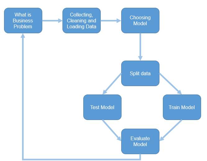
The second step in machine learning process is bout collecting (Part 2), cleaning and loading data (current part).
Azure ML has different components for data transformation (see below image ).
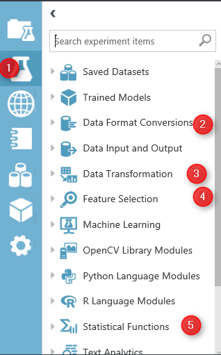
Image 1.Azure ML Data Manipulation and Transformation.
In azure ML studio, click on the Azure Experiment component (image1.1). there are different type of components that can be used for different scenario of data transformation.
in this post I will talk about “Data Transformation” (Image 1.3) component and in detail data manipulation. this component has many thing that help us to transform data, clean data and so forth.

the main part that can be used in most of Machine Learning experiments is “Manipulation” . in the below image you will be able to see the different components

Add Columns
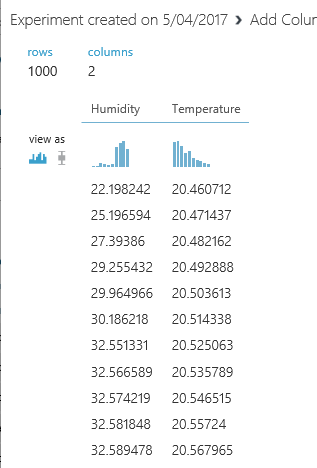
Add Columns is one of the primary type of data transformation that help you to combine two datasets. For example, imaging we have a dataset about weather Humidity and another one about the weather temperature.

there are in different data set and you want to combine them.
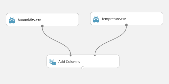
The first step is to drag and drop these two data set into the experiment area. Then connect them to the “Add Column” module (see above image).
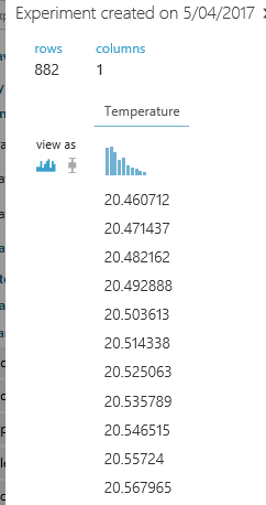
if just right click on the node bottom of the module “Add Columns” you will see that we have a dataset that have both Temperature and Humidity data in once palce.
Add rows
This component helps us to add combine rows that we have in a dataset, or combine the evaluation results. Imagine that we created an experiments that run two machine learning, we want to compare and show the result of evaluation for each of them.
I am going to explain this component via an existing Experiment in Sample experiment in Azure Ml studio. To start, click on the experiment option (below image), then click on the sample option (number 2), then in the search area type the “Binary Classfication: Credit risk prediction” and just click on the sample to open it.

when you open the sample do not freak out! I will talk about all other components in this experiment later in Machine learning parts. just click on the Run at the bottom of the page and just look at the “Add rows” and evaluation models components.

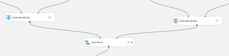
as you can see in below image, we have two “Evaluate model” components (will talk about it in Machine learning part).
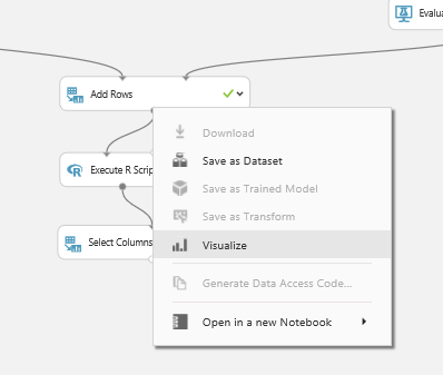
First, visualize the “Evaluation Model” component by right clicking on the node at the bottom of the component (See below image).
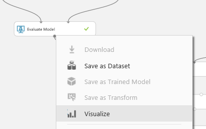
Then click on the “Visualize” option (above image). and you will see the evaluation result page. just scroll down to reach the text part of the evaluation result as below. This component show the accuracy of the model to us with charts and numbers. However, in add rows component only the numbers and data will be shown.

However, the node “Evaluation Model” has some also data output, to see just data not the graphs, I am going to drag and drop another component to model name as “Convert to Dataset” as below. I just did this to show you the real data that will pass to the “Add Rows” component.
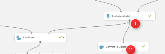
just connect it to the evaluation model and then right click on the bottom of “Convert to Dataset” component to visualize the data (see below picture)
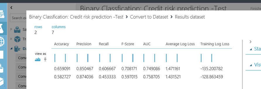
we have the same for other “evaluation model” component as below
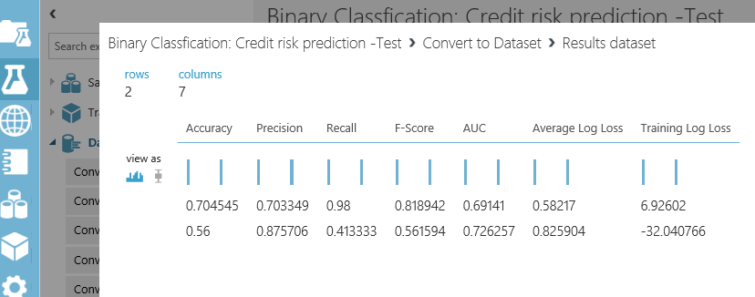
“Add Row” component will merge these information. As you can see in above picture, the row data of the “evaluation model” is just 2 rows with 7 columns. that each of them try to explain the accuracy of model to end user. we want to compare the results of these two algorithms with other ones. Hence,to see the results, just right click on the bottom of the “Add Rows” component, then click on the “Visualize” option.
the below picture shown to you. as you can see “Add Rows” has merged these data in one place

and we able to compare the result together. I will talk about the evaluation model later in Machine learning part.
In Next post I will talk about the other component for data transformation.