New Series of Time Series: Part 1

In this new series I am going to look at the time series models and how we able to use them for forecasting data.

The first need in timeseries data is to have a series of data for years or for some qurdant.

imagin that we have a time series data on birth rate from 1946 december to 1956 (file http://robjhyndman.com/tsdldata/data/
nybirths.dat) .

1- Read Data

this data has some information about the number of birth in each month, moreover, it does not have the date

we are going to read data from an url, as data is in “dat” format, we using “scan” function to read it as below :

births <- scan("http://robjhyndman.com/tsdldata/data/nybirths.dat")

the result of runnig this code in Rstudio: “168 items” items have been found.

2-Convert to Timeseries Object

to work with timeweires data first we should convert them in a Time series Object by using “TS” function in Rstudio. TS function get the data and convert a numeric vector into an R time series object.  in this example, we just add the data with out the time into “births” variable. However, we need the date like start and enddate. 

TS function also gets some inputs such as: “Frequency” “Start” and “End” : TS(Data, frequency, start, end)

Frequency:as its name said, it look for the number of intervals for stored data, for instance for a year we set the value as 12, for quarter we set value as 4.

for instance for number of birth in Newyork we should write below codes to convert data into Timeseries :

ts(births, frequency=12, start=c(1946,1))

the births is the data that we collected, the frequency is 12 as in each year we have 12 months, from Jan to Dec. Moreover,  the start of the data was from 1946 Jan, so we have c(1946,1) as a vector for start date.

now I am using the “Plot” function to draw the time series data as below

plot(ts(births, frequency=12, start=c(1946,1)))

the chart will be as below :

Before heading to analysis the chart, lets look at the other example:

I am going to look at the data for milk production for each month from 1962 to 1975, we are going to draw a time series plot for this data.

first I import data into R studio as below

milk<-monthly_milk_production_pounds_p

then we convert tha value into a timeseries object and plot it

milkTS<-ts(milk)
plot.ts(milkTS)

the result will be as below

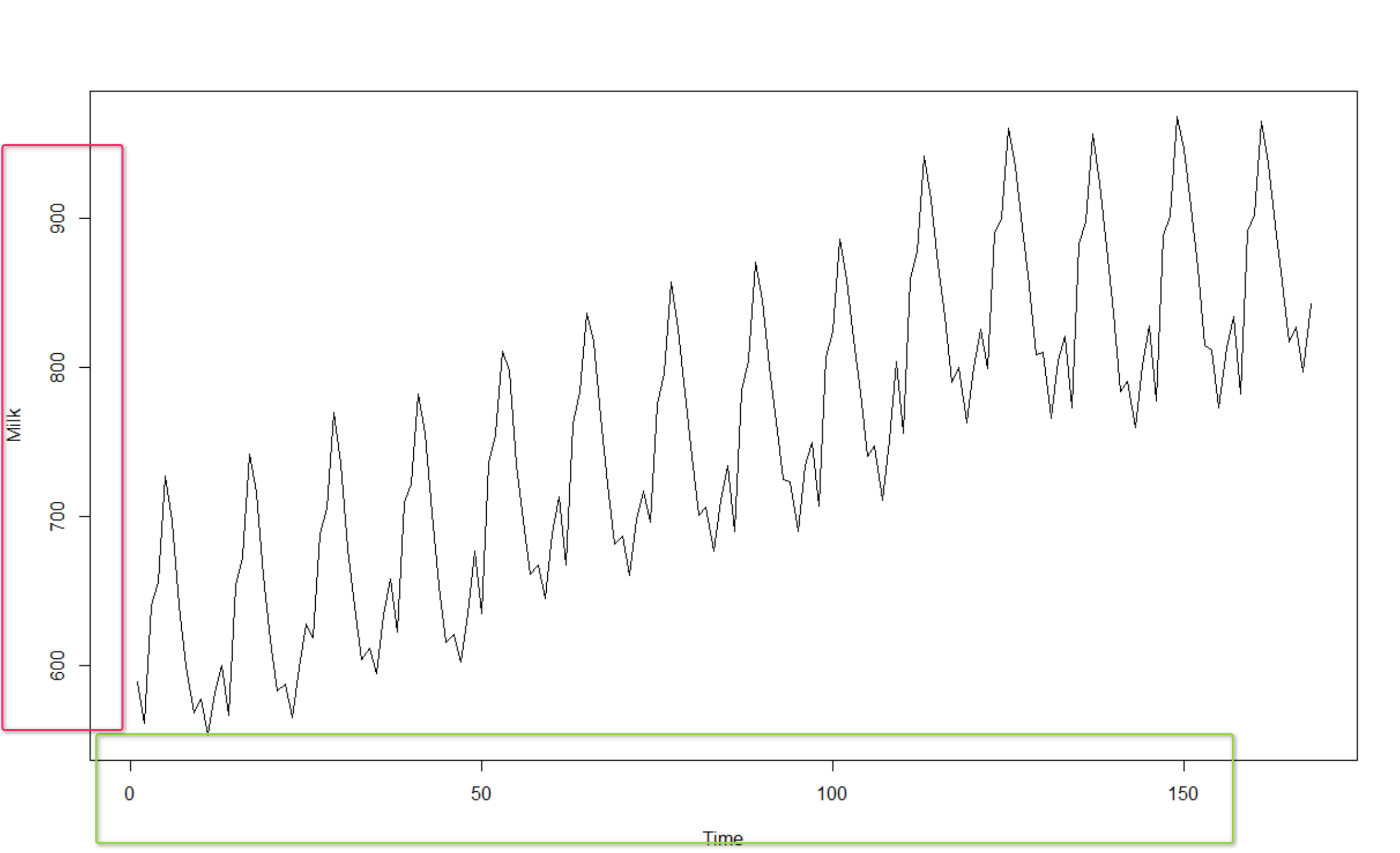
However, the timing is not correct, so I am going to add frequency and start and end time to the data as below

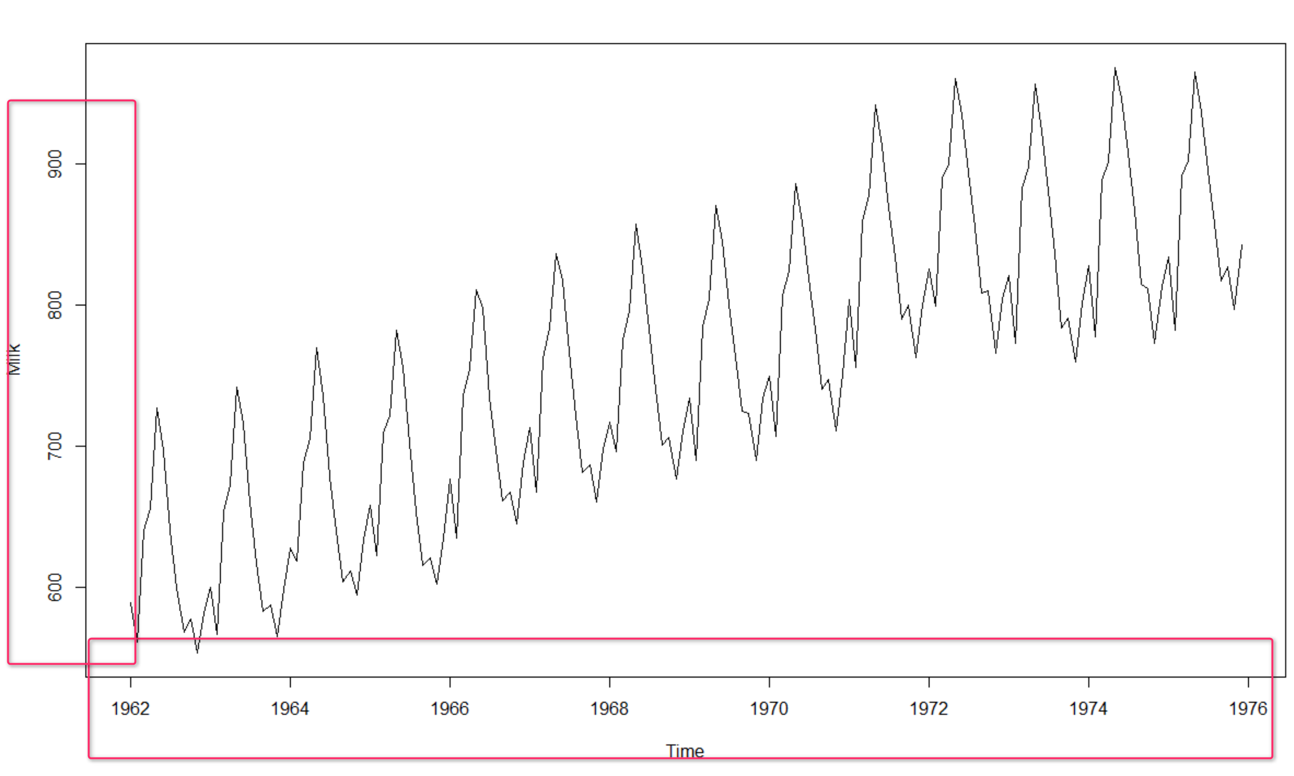
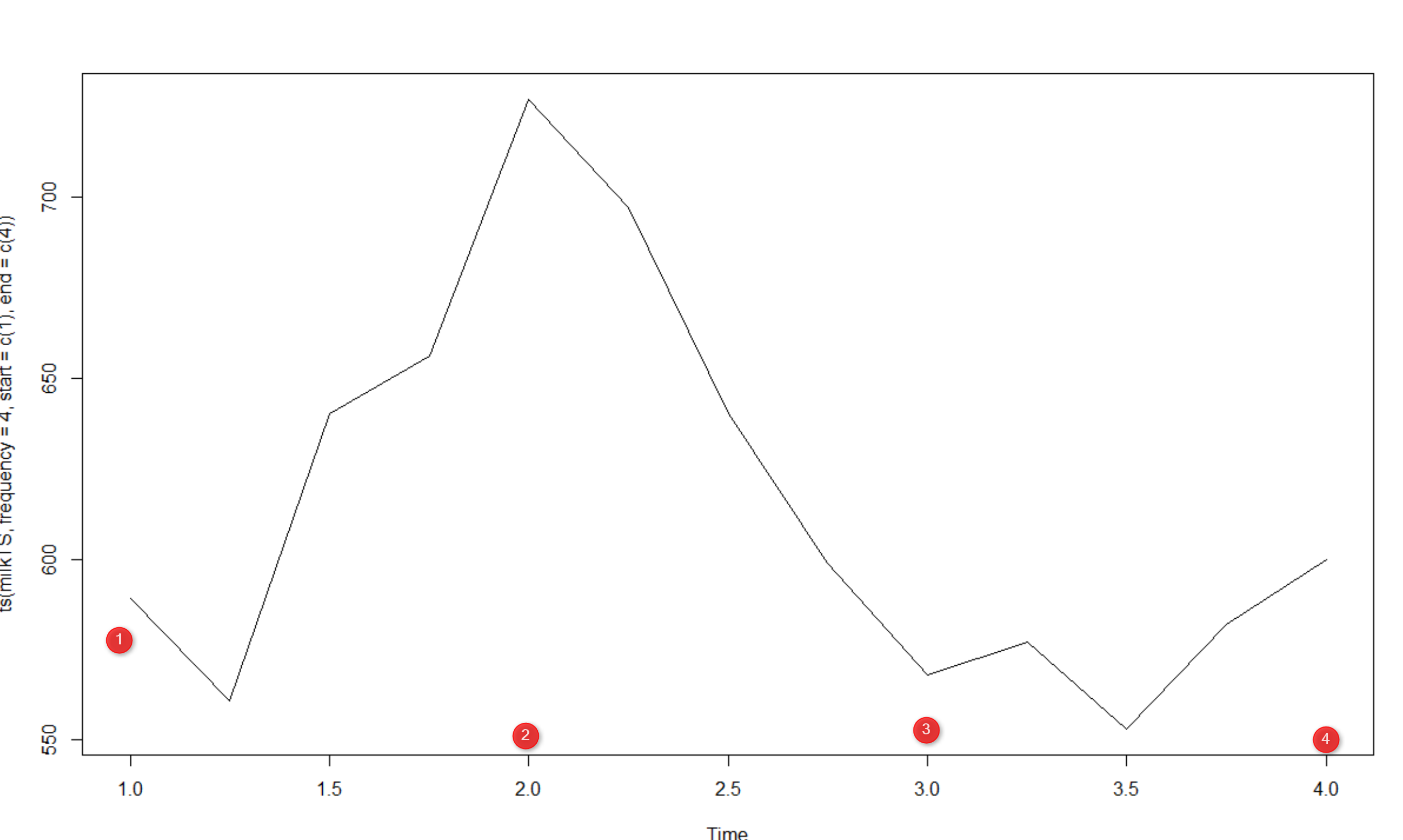
plot(ts(milkTS,frequency=12,start=c(1962,1),end = c(1975,12)))

so, the chart will be like below :

3-Timeseries Components

as you can see in above charts, these charts talk about different things in one picture

1- Trend

2- Seasonality

3- Irregular component

Trend

trend is about “long-term increase or decrease in the data” . for instance in the milk production we can see there is increase trend in production.

Seasonality

A seasonal pattern when data is influence by seasonal or any order. for instance, in above picture, you see in all years in the second quarter  milk production is high and then in the third quarter is the lowest one (see below ), and this trend is same in all years

Irregular component

there is no trend, seasonality in data

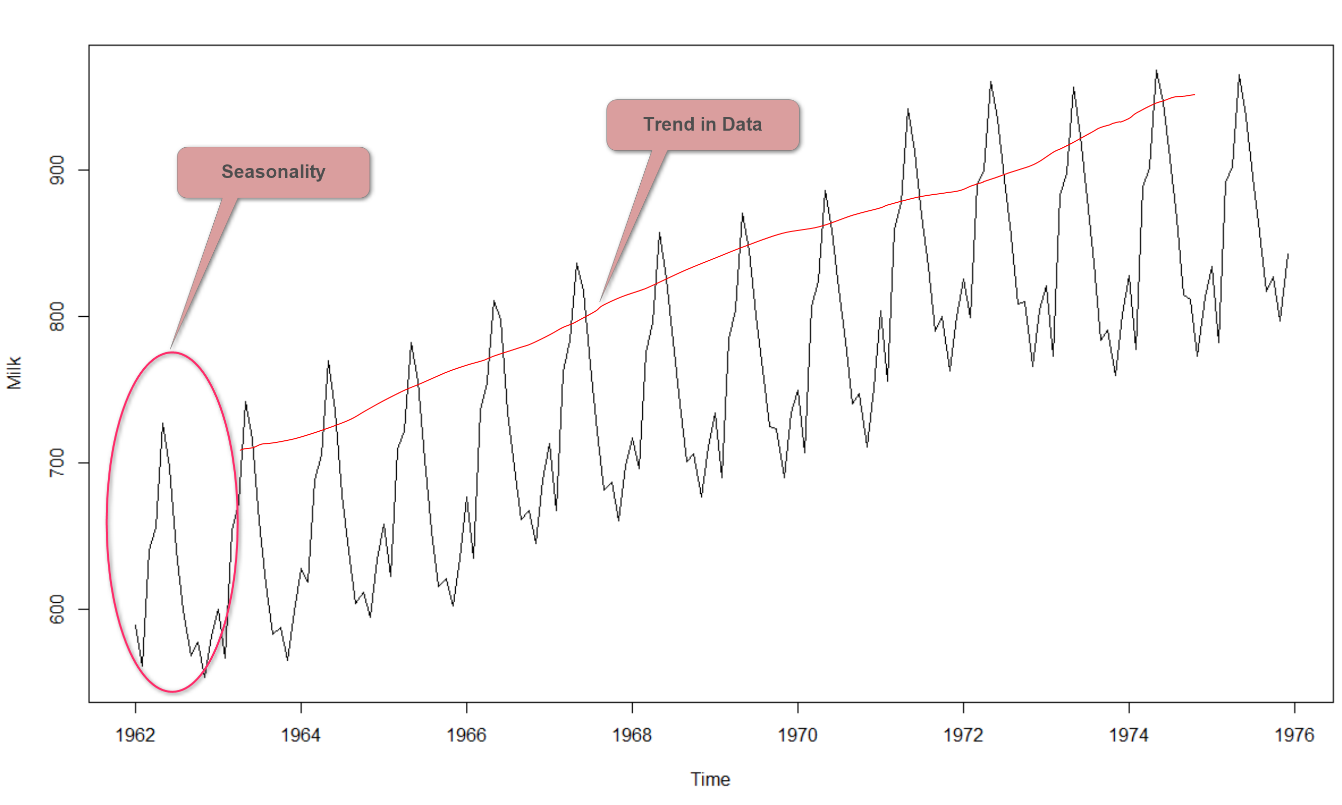
Combinations

In some of time series example we able to see both seasonality and trend (see the below picture).

we able to decompose these components:

Decompose non seasonal Data: Trend data +irregular Data

Decompose Seasonal Data : Seasonal Data +Irregular Data

In the above picture, we have both Trend and Seasonality data. (charts shows an increase rate and also a seasonal pattern)

so we able to decompose them using a command name “Decompose”

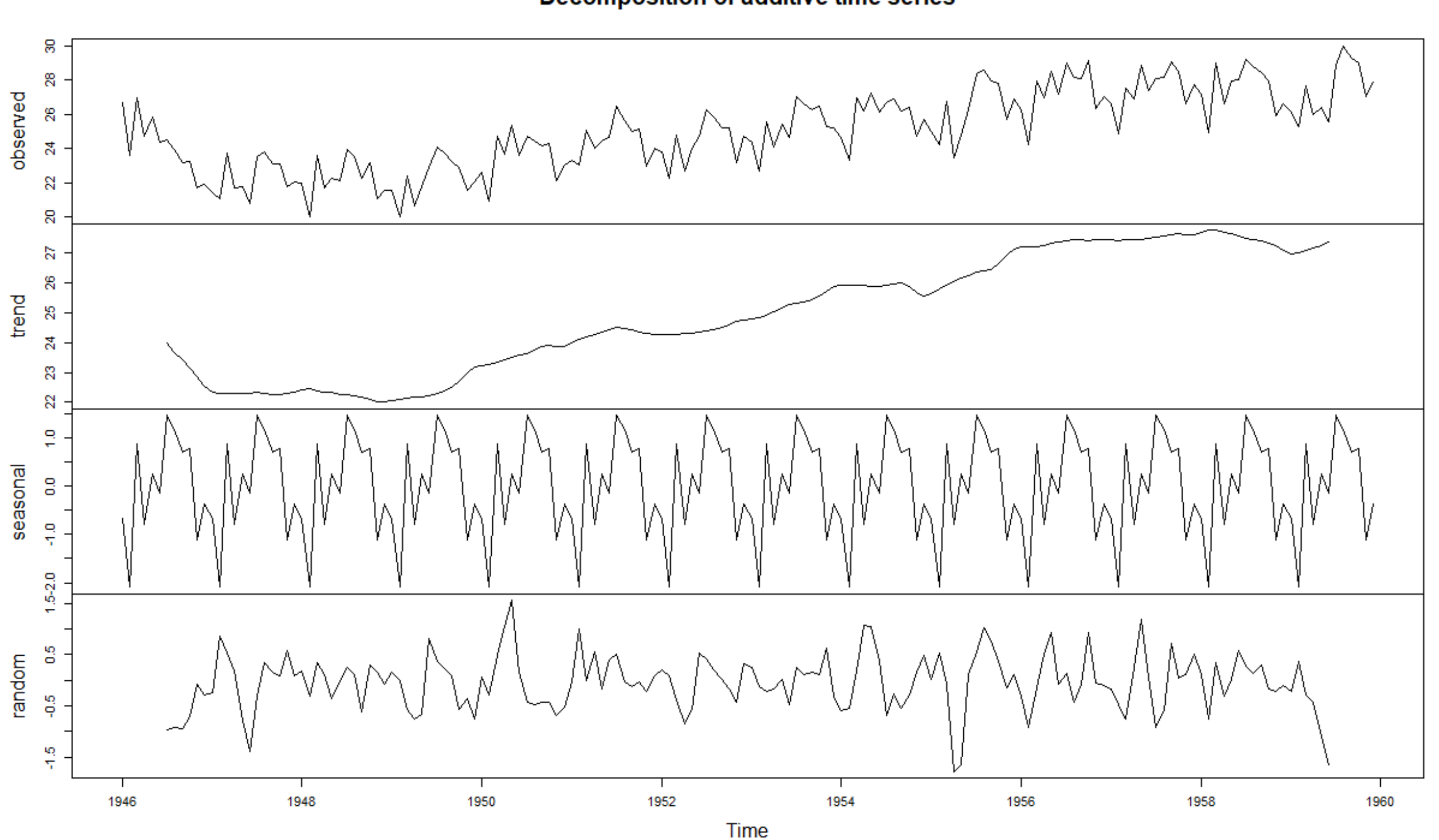
milkdecompose<-decompose(Milkts)
plot(milkdecompose)

we got the below charts

as you can see in the above picture, the milk production has 3 main parts : trend, seasonal and random.

in the next part I will talk about the timeseries models more deeply.

[1] Book:http://a-little-book-of-r-for-time-series.readthedocs.io/en/latest/src/timeseries.html

[2] data about the birthrate:

[3] data about the milk production : https://datamarket.com/data/set/22ox/monthly-milk-production-pounds-per-cow-jan-62-dec-75#!ds=22ox&display=line

[4]https://onlinecourses.science.psu.edu/stat510/?q=node/70

Leila Etaati

Trainer, Consultant, Mentor

Leila is the first Microsoft AI MVP in New Zealand and Australia, She has Ph.D. in Information System from the University Of Auckland. She is the Co-director and data scientist in RADACAD Company with more than 100 clients in around the world. She is the co-organizer of Microsoft Business Intelligence and Power BI Use group (meetup) in Auckland with more than 1200 members, She is the co-organizer of three main conferences in Auckland: SQL Saturday Auckland (2015 till now) with more than 400 registrations, Difinity (2017 till now) with more than 200 registrations and Global AI Bootcamp 2018. She is a Data Scientist, BI Consultant, Trainer, and Speaker. She is a well-known International Speakers to many conferences such as Microsoft ignite, SQL pass, Data Platform Summit, SQL Saturday, Power BI world Tour and so forth in Europe, USA, Asia, Australia, and New Zealand. She has over ten years’ experience working with databases and software systems. She was involved in many large-scale projects for big-sized companies. She also AI and Data Platform Microsoft MVP. Leila is an active Technical Microsoft AI blogger for RADACAD.