
Part 1 of 3 Using RANKX in calculated measures
Part 2 of 3 Using RANKX in calculated columns
This article concludes my epic series detailing how to use the RANKX function in DAX. In this episode, Frodo finally reaches Mt. Doom and successfully uses RANKX to find the best path into the mountain and complete his journey. What you probably don’t appreciate is when Frodo returned home, the first thing he did was create a Power BI Report about his adventures, which J. R. R. Tolkien later converted into a successful book and movie.

The first 2 articles covered how to use the RANKX function with calculated columns and calculated measures. This article will focus on the mysterious and optional third parameter and attempt to break down what it does and when it might be useful.
The official documentation from Microsoft suggests the syntax for the RANKX function is as follows:
RANKX(<table>, <expression>[, <value>[, <order>[, <ties>]]])
I will focus on the optional <value> parameter.
RANKX is an iterator function, which means it will run a loop as many times as there are rows in the <table> passed as the first parameter. Each time the RANKX function is calculated, it evaluates the DAX code provided as the <expression> and builds a sorted list to establish the rank order. The value returned by <expression> for the current context of the call to the RANKX function is then used to find the position in the sorted list, so long as the <value> parameter is not used. It is the position in the list that the RANKX function returns.
I will use the same data-set used in the first two articles to demonstrate.
The DAX code to generate the sample data is the following calculated table:
Table =
    DATATABLE
        (
        "Category"      , STRING ,
        "Sub Category"  , STRING ,
        "Date"          , DATETIME ,
        "My Value"      , INTEGER ,
            {
            {"A","A1","2018-01-01", 2},
            {"A","A2","2018-01-02", 4},
            {"A","A3","2018-01-03", 6},
            {"A","A4","2018-01-04", 6},
            {"B","B1","2018-01-05",21},
            {"B","B2","2018-01-06",22},
            {"B","B2","2018-01-07",23},
            {"C","C1","2018-01-08",35},
            {"C","C2","2018-01-09",35},
            {"C","C3","2018-01-10",35}
            }
        )
The following calculated column can be added to the above calculated table:
RANKX as Column =
    RANKX (
        'Table',
        'Table'[My Value],
        -- Placeholder --
        ,
        ASC
        )
Once added, we see the following output now includes a column ranking for each row in ascending order based on the value in the ‘Table'[My Value] column. This includes some tied results. I have some detail on how to deal with tied results in the first two blogs in this series.
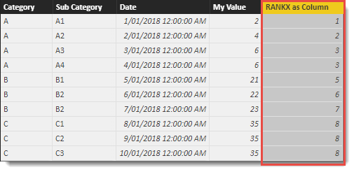
So far so good. The calculated table added to our model had 10 rows so when the calculated column was added, each row in the table runs the code contained in the calculated column using each rows specific filter context. In this example the RANKX function will be executed 10 times.
Logically, each execution of the RANKX Function will iterate 10 times and produce 10 lists. The only difference between each execution of RANKX is when it comes to the end when the value used to find the position inside the sorted list of values is different.
To help debug and see what is going on inside each RANKX function, the CONCATENATEX function can be used as a substitute to help visualise the internal loops of an iterator function. The calculated column below, is using CONCATENATEX in place of RANKX so we can see the output as text.
CONCATENATEX as Column =
    CONCATENATEX(
        'Table',
        'Table'[My Value],
        ", "
        )
The new calculated column appears at the end of the table and shows text generated by the iterator function for each cell in the table. One sorted, I highlighted the position in the list for each row based on the value that would be used as the 2nd paramenter <expression>. The position number (highlighted by a red outline) in the list is what is returned by the function. In the top row, the first value in the list (left to right) matches the value in the My Value column, so RANKX returns a 1.

Let’s now add some code to our RANKX function to override the output for one of the rows.
RANKX as Column with override =
    RANKX (
        'Table',
        'Table'[My Value],
        IF(
            'Table'[Sub Category] = "A2" ,
            -- THEN --
            99 ,
            -- ELSE
            'Table'[My Value]
            )
        ,
        ASC
        )
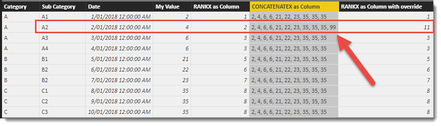
I have used an IF statement as the third parameter to check if the current row belongs to Sub Category = “A2”. Any row matching this criteria has a value of 99 generated. The original list generated naturally by the iterator (2, 4, 6, 6, 21, 22, 23, 35, 35, 35) is then checked to see if it contains the number 99 and if it finds a match, this position is used as the output for the RANKX function.
However, if the new value (99) is not found in the list, which is what has happened here, the <value> of 99 is added to the list and the list is re-sorted. The new list to determine ranking positions is now as follows (2, 4, 6, 6, 21, 22, 23, 35, 35, 35, 99). Note the 2nd position of 4 still exists, so ranking values are NOT shuffled up to account for the re-position. The number 99 happens to be the 11th position of our list so a number 11 is returned as the output of the RANKX function for the 2nd row of the table.
The image shows the extended version of the list in row two. This row has a slightly longer list than the others because it was the only row that needed to add a new value to the list and re-sort. For all the other rows, the if statement returned a value that already existed in the original list. This explains why the RANKX function is not shuffled up for the rows below our A2 row. They independently found their list positions based on the list shown for their respective row.
If we tweak the calculation to override to a 0 (zero) instead of a 99 we see the following:
RANKX as Column with override to zero =
    RANKX (
        'Table',
        'Table'[My Value],
        IF(
            'Table'[Sub Category] = "A2" ,
            -- THEN --
            0,
            -- ELSE
            'Table'[My Value]
            )
        ,
        ASC
        )
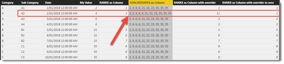
You will see here, that for the highlighted row, the text list now generates a 0 (zero) to be added to the iterator generated list (but just for this row only!). When it comes to finding the position in the list, it is in the first spot, so returns a 1.
The top row also returns a 1, because as far as it is concerned, the <value> of 2 happens to be in the first position of its list so also returns a 1.
Clear as mud? At the very least, I hope this explanation helps to clarify the logical workings of the RANKX function and in particular, what the effect is to result when you use the <value> parameter.
Now let’s override a group of rows by setting any with a Category of “B” to use a <value> of 15.
RANKX as Column with override to 15 =
    RANKX (
        'Table',
        'Table'[My Value],
        IF(
            'Table'[Category] = "B" ,
            -- THEN --
            15,
            -- ELSE
            'Table'[My Value]
            )
        ,
        ASC
        )
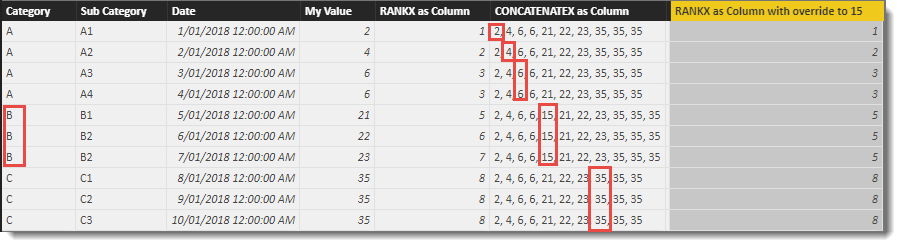
Here is the result. I have highlighted in each row the position in the iterator generated list once the <value> has been applied. Note that only the three rows belonging to Category “B” are using a slightly longer list and hence the RANKX value generated in the calculated column reflects the list position when counting from the left.
This hopefully helps explain a little more about how RANKX works and in particular, the effect using the third parameter has on the result. The next question is, when might this parameter be useful?
One reason to use the <value> parameter might be to show how your <value> might be ranked when used in a different table. e.g. you have a list of products showing sales and ranking for 2017 data, and you might also want to show how the 2017 sales would have been ranked if compared with a list of product sales for 2016.
The examples up to this point used the same table for outer and inner tables for the iterator function. The outer table is the physical table we are adding the calculated column to. The inner table is the first <table> parameter used in the calculation.
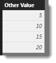
Let’s add a small table to the data model and use this in a new calculation. The code to add the new table is :
Other Table =
    DATATABLE
        (
        "Other Value"      , INTEGER ,
            {
              {  5 },
              { 10 },
              { 15 },
              { 20 }
            }
        )
This adds a 4 row, single column table that should appear as follows:
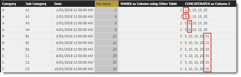
Now if we add a calculated column to the first table in our model using the following code :
RANKX as Column using Other Table =
    RANKX (
        'Other Table',
        'Other Table'[Other Value] ,
        'Table'[My Value],
        ASC
        )
The value returned in the fifth column shows the position of the value in the forth column in the list of values in the right column.
In this example, the RANKX function loops through each row in the ‘Other Table’ and generates a list of values using the [Other Value] column. There are only 4 rows in ‘Other Table’, so the initial version of the list only has four values (5 , 10 , 15 , 20).
In each case, if the value being passed in the third parameter doesn’t exist in the list, the value is added and the list is then sorted. It is the position in the final list of the value that is returned by the RANKX function.
For each row in the table below the right most column is showing the final iterator generated list for each RANKX call.
This would not be a common scenario, so if you are wondering if you need to use the third parameter at all, the chances are you don’t. However, if you need to force an item to the top or bottom of a ranking list, or need to compare a current value with a previous list – then you might need to come back and re-read this article.
And that is how Frodo defeated the forces of Mordor and everyone lived happily ever after. Except for Sauron, who was the original author of the RANKX function. 🙂
Ranking without using RANKX
A nice alternative to using RANKX to generate ranking functions is to use the COUNTROWS function. When used with a filter (which is also an iterator), it can be used to simply count the rows that are higher, or lower that the current row based on a value.
One syntax when used in a calculated column is
COUNTROWS as RANK =
VAR CurrentRowValue = 'Table'[My Value]
RETURN
    COUNTROWS(
        FILTER(
            'Table',
            'Table'[My Value] < CurrentRowValue)
            ) + 1
And when added to our table we see the following result. The calculated column simply counts the rows of the table generated by the FILTER statement. As you can see, the two right most columns return exactly the same values.
The COUNTROWS approach is logically similar to the RANKX, in that FILTER is also an iterator. For a future article, I might spin up a much larger data-set to test the performance characteristics between the two approaches.


hi Philip,
nice article. very helpful.
one question, how do you use CONCATENATEX to examine the internal loop of RANKX, if 3rd parameter is used (in your example, override certain value)?
thanks.
Very good article, and you picked nice example which covers many scenarios