Aggregations are speeding up the model. However, the aggregated table is not just one table; It can be multiple layers of aggregations. Aggregation by Date, aggregation by Date and Product, aggregation by Date and Product and Customer. Multiple layers ensure that you always have the best performance result possible, and you only query the DirectQuery data source for the most atomic requests. Let’s see how this process is possible and helpful. If you like to learn more about Power BI, read the Power BI book from Rookie to Rock Star.

To learn more about aggregations, read the article series here:

• What is aggregation in Power BI?
• Step 1: Create the aggregated table
• Step 2: Dual Storage Mode
• Step 3: Configure Aggregation Functions

Sample model

Our sample data model (which we built in the previous blog post), has already an aggregated table; Sales Agg, and one DirectQuery fact table; FactInternetSales.

In this example, we will add more aggregations to the model.

Second Aggregation Layer

Create the aggregation table

The second aggregation layer I will add in this example is including Promotion also into the grouping options. Here is my group by settings for my second aggregation table in Power Query. If you are interested to learn in detail how the aggregated table can be created, read my other blog post about creating the aggregated table.

Set up relationships

Then load the table into Power BI, and create relationships to DimDate, DimCustomer, DimProductSubcategory, and DimPromotion.

Dual Storage Mode

Set the Storage mode of DimPromotion to Dual. It is very important to use the Dual storage mode. With this setup, Power BI for aggregation-based analysis will use the in-memory copy of the DimPromition, and for the atomic transaction levels, it will use the DirectQuery version of it. Read my blog post here to learn all about the Dual storage mode.

Manage Aggregations

After setting up relationships and storage modes, you need to Manage Aggregations on the Sales and Promotion Agg table (this is our second aggregation table);

Everything is similar to the Aggregation setup we had before for the Sales Agg table. For this one, the only addition is the Group By action on PromotionKey.

Precedence Setup

When you have multiple layers of aggregation, you must set up their precedence. The aggregated table you want to take the highest priority should have the highest precedence. In this case, Sales Agg can be 1, and Sales and Promotion Agg can be 0.

Testing the result

With the above setup, you can have visualizations that use promotions, Customer, Date, and ProductSubcategory and still be sourced from the aggregation. Here is an example;

This kind of visualization will not send any query to the DirectQuery source;

How about Precedence of Execution?

When you have multiple aggregation layers, which one runs first is important. As an example, let’s assume some numbers. These are not real numbers; these are just numbers to help you understand the scenario. The big fact table (FactInternetSales) uses DirectQuery mode and has 250 million rows. And the Sales Agg table has only 10,000 rows. But the Sales and Promotion Agg has 1,000,000 rows. In such a scenario, when you are querying something that can be answered with the table with 10K rows (Sales Agg), you have to do so because it would be much faster than the table with 1M rows (Sales and Promotion Agg). Therefore, we need to set up the precedence of execution. Smaller aggregation tables should be the source of analysis first.

Query hits the First Aggregated Table in the Memory.

Here is a visual in the Power BI Page using Gender (from DimCustomer) and SalesAmount (from FactInternetSales);

A visual like the above will be querying not the FactInternetSales table but the aggregated table behind the scene. In this case, it will query the Sales Agg table. Here is behind the scene query sent to the Vertipaq engine (result generated from SQL Profiler);

In this example; the query hits the first aggregated table in the memory;

Query hits the second aggregated table in the memory

Here is another visual that uses EnglishPromotionType (from DimPromotion), and SalesAmount (from FactInternetSales);

And the result this time cannot be fetched from the Sales Agg table (because DimPromotion is not there as the group by function), so it will be queried from the second aggregated table: Sales and Promotion Agg.

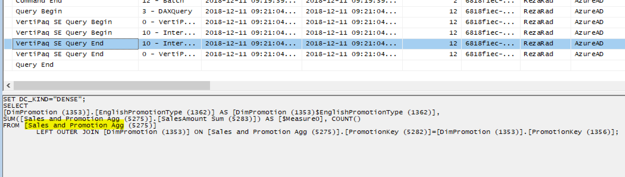
In this instance, the query hits the second aggregated table in the memory;

Query hits the DirectQuery table in the source

As the last visual in this example, the Visual below uses EnglishProductName (from DimProduct), and SalesAmount (from FactInternetSales);

and the result this time cannot be fetched from any of the aggregated tables, so it comes directly from the DirectQuery source table: FactInternetSales

In the last example; the query hits the DirectQuery table in the data source:

Power BI is switching nicely between layers of aggregated tables without you noticing it. All the above operations are happening behind the scene. The user will feel that one table (FactInternetSales) is serving all queries, and the query response time will be super fast (with the help of aggregations).

Summary

Aggregation can be implemented on multiple levels to speed up the performance faster and faster. If a specific combination of dimension fields is used a lot in user visualisations, that combination is a good candidate for aggregation. Depending on the size of the aggregation table, precedence should be followed. Please let me know in the comments below if you have any questions about aggregations.

Previous Steps

• Power BI Fast and Furious with Aggregations
• Power BI Aggregation: Step 1 Create the Aggregated Table
• Dual Storage Mode; The Most Important Configuration for Aggregations! Step 2 Power BI Aggregations
• Power BI Aggregations Step 3: Configure Aggregation Functions and Test Aggregations in Action
• Multiple Layers of Aggregations in Power BI; Model Responds Even Faster (The current article)
• Aggregation on Import Data models

Reza Rad

Trainer, Consultant, Mentor

Reza Rad is a Microsoft Regional Director, an Author, Trainer, Speaker and Consultant. He has a BSc in Computer engineering; he has more than 20 years’ experience in data analysis, BI, databases, programming, and development mostly on Microsoft technologies. He is a Microsoft Data Platform MVP for 12 continuous years (from 2011 till now) for his dedication in Microsoft BI. Reza is an active blogger and co-founder of RADACAD. Reza is also co-founder and co-organizer of Difinity conference in New Zealand, Power BI Summit, and Data Insight Summit.
Reza is author of more than 14 books on Microsoft Business Intelligence, most of these books are published under Power BI category. Among these are books such as Power BI DAX Simplified, Pro Power BI Architecture, Power BI from Rookie to Rock Star, Power Query books series, Row-Level Security in Power BI and etc.
He is an International Speaker in Microsoft Ignite, Microsoft Business Applications Summit, Data Insight Summit, PASS Summit, SQL Saturday and SQL user groups. And He is a Microsoft Certified Trainer.
Reza’s passion is to help you find the best data solution, he is Data enthusiast.
His articles on different aspects of technologies, especially on MS BI, can be found on his blog: https://radacad.com/blog.