In the part 1, I have explained how to use R visualization inside Power BI. In the second part the process of visualization of five dimension in a single chart has been presented in Part 2, and finally in the part 3 the map visualization with embedded chart has been presented.
In current post and next ones I am going to show how you can do data comparison,  variable relationship, composition and distribution in Power BI.

Comparison one of the main reasons of data visualization is about comparing data to see the changes and find out the difference between values. This comparison is manly about compare data Over time or by other Items.

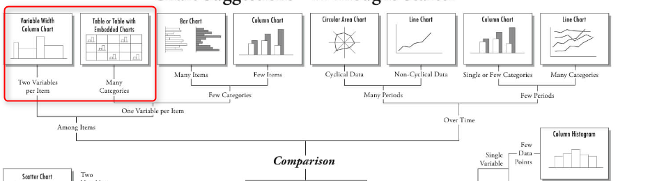
for comparison purpose most of the charts can be available in Power BI Visualization, just two of them are not :Variable Width Column Chart and Table with Embedded Chart.

In this post I will talk about how to draw a “Variable Width Column  Chart” inside Power BI using R scripts.

In the next Post I will show how to draw a Table with Embedded Chart” in the next post.
Variable Width Column  Chart

you will able to have a column chart with different width inside Power BI by writing R codes inside R scripts editor.

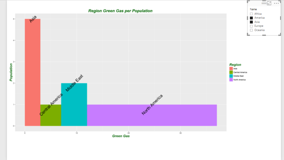
to start I have some dummy data about amount of green gas and population of each region .

in the above table, “Pop” stands for “Population” “Gas” stands for “Green Gas” amount.

to start, first click on the “R” visualization icon in the right side of the page in power bi desktop. Then, you will see a blank visualization frame in the  middle of the report. Following, click on the required fields at the right side of the report to choose them for showing in the report. Click on the ” Gas”, “Pop” and “Region” fields.

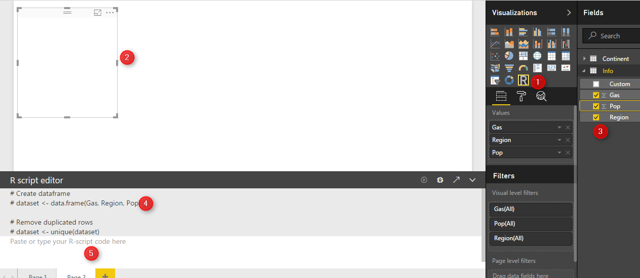
at the bottom of the page, you will see R scripts editor that allocate these three fields to a variable named “dataset”(number 4).

We define a new variable name “df” which will store a data frame (table) that contains information about region, population and gas amount.

df<-data.frame(Region=dataset$Region,Population= dataset$Pop,width=dataset$Gas)
as you can see in above code, I have used “$” to access the fields stored in “dataset” variable.

now, I am going to identify the width size of the each rectangle in my chart, using below codes

df$w <- cumsum(df$width) #cumulative sums.
df$wm <- df$w – df$width
df$GreenGas<- with(df, wm + (w – wm)/2)

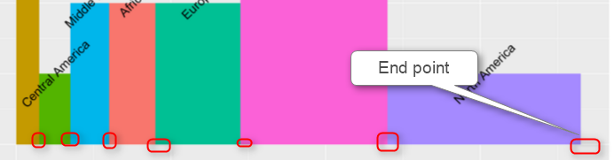
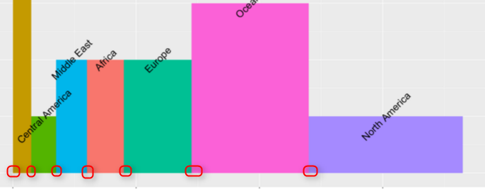
the first step is to identify the start point and end point of each rectangle.

“cumsum” a cumulative sum function that calculate the width  of each region in the graph from 0 to its width. This calculation give us the end point (width) of each bar in our column width bar chart (see below chart and table).

so I will have below numbers

so we store this amount in df$w variable.

next, we have to  calculate the start point of each bar chart (see below chart) using : df$wm <- df$w – df$width

Moreover, we also calculate the start point of width for each bar as below

Another location that we should specify before hand is the rectangle lable. I prefer to put them in middle of the bar chart.

we want the label text located in the middle of each bar, so we calculate the middle of width (average) of each bar as above and put the value in df$GreenGas. This variable hols the location of each labels.

so we have all data ready to plot the chart. we need “ggplot2” library for this purpose

library(ggplot2)

we call function “ggplot” and we pass the first argument to it as our dataset. the result of the function will be put in variable “P”
p <- ggplot(df, aes(ymin = 0))

Next, we call another function as below, this function draw a rectangle for us. this get the start point of each rectangle (bar) as “wm” and the end point of them “w” (we already calculated them in above and the third argument is the range of the “Population” number. The last argument if the colouring each rectangle based on their related region.

p1 <- p + geom_rect(aes(xmin = wm, xmax = w, ymax = Population, fill = Region))

p1

if we run the above codes we will have below chart

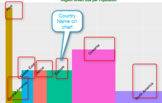
our chart does not have any label. so we need to add other layer to p1 as below .

p2<-p1 + geom_text(aes(x = GreenGas, y = Population, label = Region),size=7,angle = 45)

p2

geom_text function provides the title for x and y axis and also for the each rectangle using “aes” function aes(x = GreenGas, y = Population, label = Region).

however you able to change the size of the text label for each bar (rectangle) by adding a parameter ” size”. for instance I can change it to 10. or you can specify the angel of the label (rotate) it by another parameter as “angel” in this chart I put it to be “45” degree.

I am not still happy with chart, I want to change the title of  x and y axis and also add a title to chart. To do this, I add another layer to what I have. I call a function name “labs” which able me to specify the chart title, x and y axis name as below

p3<-p2+labs(title = “Region Green Gas per Population “, x = “Green Gas”, y = “Population”)
p3

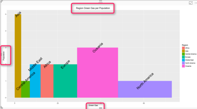
the problem with chart is that the title and text in x or y axis is not that much clear. as a result I define a them for each of them. to define a theme for chart title and the text I am going to use a function name ” element_text”.

this function able me to define some theme for my chart as below:

blue.bold.italic.10.text <- element_text(face = “bold.italic”, color = “dark green”, size = 10)

so I want the text (title chart , y and x text) be bold and italic. also the color be “dark green” and the text size be 10.

I have defined this theme. now, I have to allocate this theme to title of chart and axis text.

to do this, I call another function (Theme)and add this as another layer. Theme function I specify the axis title should follow the rules and theme I created in above code  “blue.bold.italic.10.text” . the second argument in “theme” function allocated this created theme to the chart title as below

p4<-p3+theme(axis.title = blue.bold.italic.10.text, title =blue.bold.italic.10.text)

p4

There are other factor that you able  to change them by adding more layers and function to make your chart better.

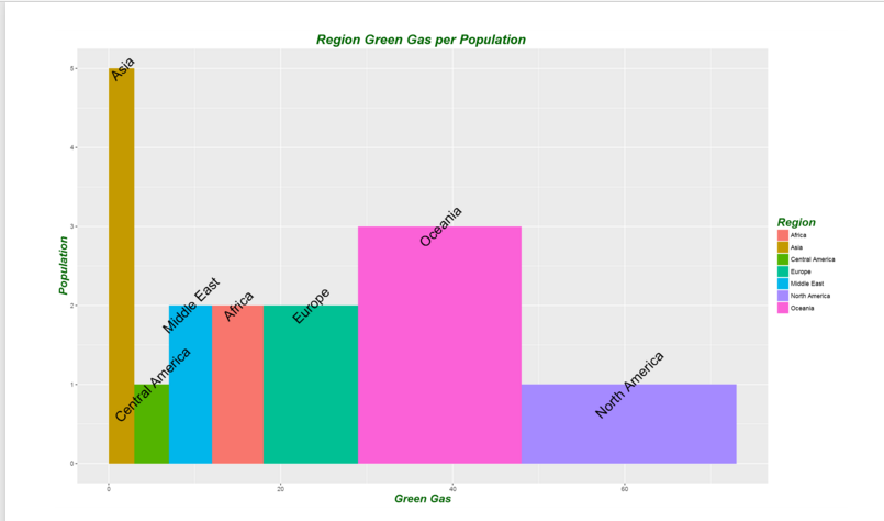
now I want to analysis the green gas per each continent. so I am going to add another slicer to my report to check it. so for example I just want to compare these numbers for “America” and “Asia” continent in my chart. the result is shown in below chart.

the overall code would be look like below :

df<-data.frame(Region=dataset$Region,Population= dataset$Pop,width=dataset$Gas)
df$w <- cumsum(df$width) #cumulative sums.
df$wm <- df$w – df$width
df$GreenGas<- with(df, wm + (w – wm)/2)
library(ggplot2)
p  <- ggplot(df, aes(ymin = 0))
p1 <- p + geom_rect(aes(xmin = wm, xmax = w, ymax = Population, fill = Region))
p2<-p1 + geom_text(aes(x = GreenGas, y = Population, label = Region),size=7,angle = 45)
p3<-p2+labs(title = “Region Green Gas per Population “, x = “Green Gas”, y = “Population”)
blue.bold.italic.10.text <- element_text(face = “bold.italic”, color = “dark green”, size = 16)
p4<-p3+theme(axis.title = blue.bold.italic.10.text, title =blue.bold.italic.10.text)
p4

I will post the Power Bi file to download soon here.

Download Demo File

[1]https://i1.wp.com/www.tatvic.com/blog/wp-content/uploads/2016/12/Pic_2.png

[2]http://ggplot2.tidyverse.org/reference/geom_text.html

[3]http://stackoverflow.com/questions/14591167/variable-width-bar-plot

Leila Etaati

Trainer, Consultant, Mentor

Leila is the first Microsoft AI MVP in New Zealand and Australia, She has Ph.D. in Information System from the University Of Auckland. She is the Co-director and data scientist in RADACAD Company with more than 100 clients in around the world. She is the co-organizer of Microsoft Business Intelligence and Power BI Use group (meetup) in Auckland with more than 1200 members, She is the co-organizer of three main conferences in Auckland: SQL Saturday Auckland (2015 till now) with more than 400 registrations, Difinity (2017 till now) with more than 200 registrations and Global AI Bootcamp 2018. She is a Data Scientist, BI Consultant, Trainer, and Speaker. She is a well-known International Speakers to many conferences such as Microsoft ignite, SQL pass, Data Platform Summit, SQL Saturday, Power BI world Tour and so forth in Europe, USA, Asia, Australia, and New Zealand. She has over ten years’ experience working with databases and software systems. She was involved in many large-scale projects for big-sized companies. She also AI and Data Platform Microsoft MVP. Leila is an active Technical Microsoft AI blogger for RADACAD.