

Decomposition Tree allows you to visualize the data regarding various dimensions. It is all about the aggregation of data and drills down.
In the first post about this feature, I am going to show how this works for a simple decomposition task, in the next posts, I will show you how embedded AI in this visual can be useful.
To start to work with this visual, make sure you have the latest version of the Power BI desktop in your machine
Also, as still, the decomposition tree is a Preview feature, if you could not see it, need to go to the File–> Option and Setting –>Option–>Preview Feature and choose the Decomposition tree visual.
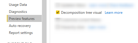
Then close and reopen Power BI desktop to be able to see the visual in Visualization panel

In the next step, I am going to use the dataset for the house price to analyze, you can download from here.
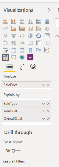
then load the data using get data option. Click on the decomposition visual. In the Analyse text box, choose the sale price, for the Explained by I select the Sale type, YearBuild, OverAllQual
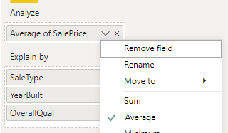
For the first experiment, I am going to change the sales price from the sum to the average amount.
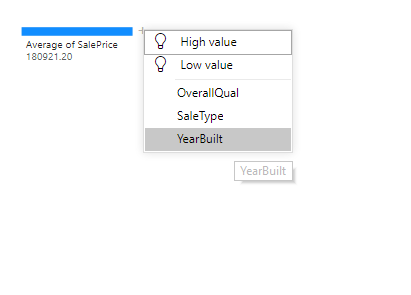
next in the visualization, you should see the bar with a total average of the house sale price. if you click on the Plus sign, you able to see couple of options. the high value and low value related to AI feature that I will explain next posts. Moreover, you able to see other fields. In this stage, we are going to see
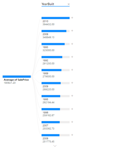
“What is the decomposition of the Sales Proces for each year so click on the Year Build.
In the next stape, you should see the decomposition as below for each year we able to see the average of the sale price so, in 2010, we have the highest sales price, next in 2008 and then 1893.
Note
The sum of the sale price you can see under the YearBuild, the sum of the column is equal to the total sale in the First Node.
So, for instance, for Overall quality, from 1 to 10 the sum of the sales price for all house quality conditions is equal to the first node that is the total sale price.

Now imagine you want to go a bit further and analyze the average of the sales price by each year then based Sale Type.
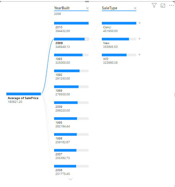
In the next step, you will see we can see the decomposition of the data based on the sales type and year build in 2008 and what sort of the sale type we have the average of the sale price.
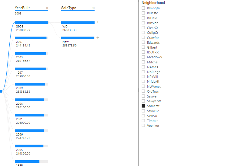
Next, you can add a slicer for the neighborhood selection to analyze in each neighborhood how much was the sale price and what was the main sale type. Choose a Neighborhood for the Somerst then you can see the in 2008 the average price was 258000 with two sales type as WD and New.
Check out the video from here