
In the last posts, I have explained the main concepts behind the Timeseries (Post 1) and in the second one a simple forecasting approach name as “Exponential Smoothing” has been proposed Post 2.
In this post I am going to show how to do see the error of forecasting and also how to forecast when we have trend and no seasonality.
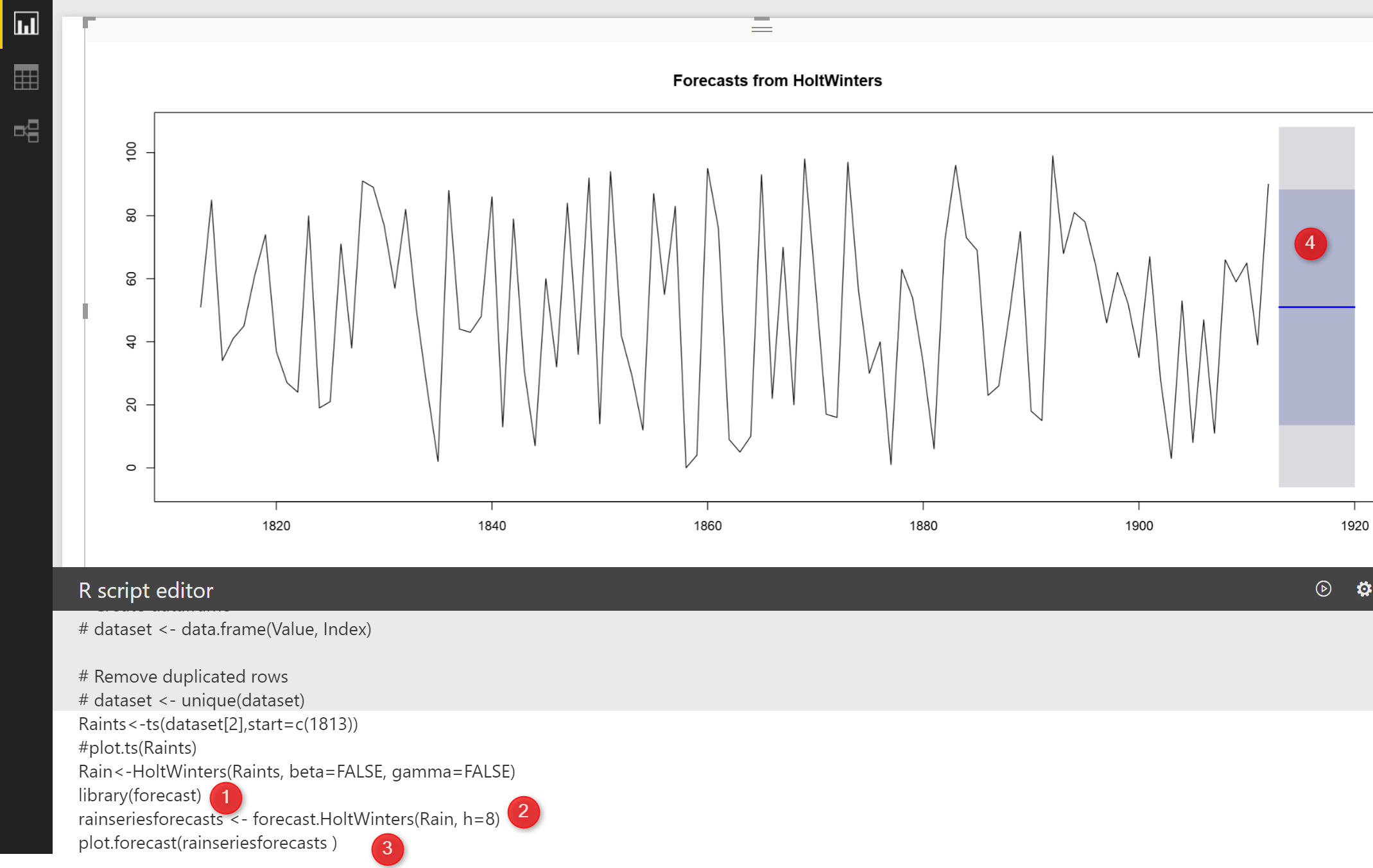
In the last post, I have used “Holtwinters” with Rain dataset and forecasting 8 event in front.
Raints<-ts(dataset[2],start=c(1813))
#plot.ts(Raints)
Rain<-HoltWinters(Raints, beta=FALSE, gamma=FALSE)
library(forecast)
rainseriesforecasts <- forecast.HoltWinters(Rain, h=8)
plot.forecast(rainseriesforecasts )
the resulr was below
Doing any prediction and forecasting should be evaluated.
So what is evaluation ?evaluation in forecasting means we are going to compare the predicted value with real world to see how much they have differences.
lower difference better!
In dataset “rainseriesforecasts” we have a column name “residuals”. This column stores the error for each data row,
so if in R studio I run the below code
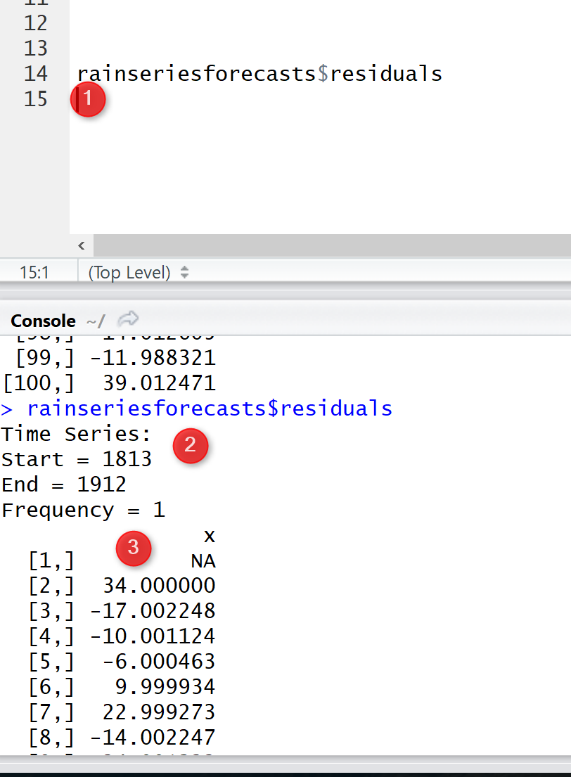
So as you see, the output is the error amonth we find for all the rows from 1813 to 1912.
There eshould be some analysis on how the error is correlated to each other, but I am not going to talk in this post.I write a post about the “ARIMA” .
Now I am going to do some more experiemnt, in the last time serie.
In the last example we donot have any trend or any seasonality.
Now, imagin we have a time series that can be described using an additive model with increasing or decreasing trend and no seasonality, you can use Holt’s exponential smoothing
Holt’s exponential smoothing
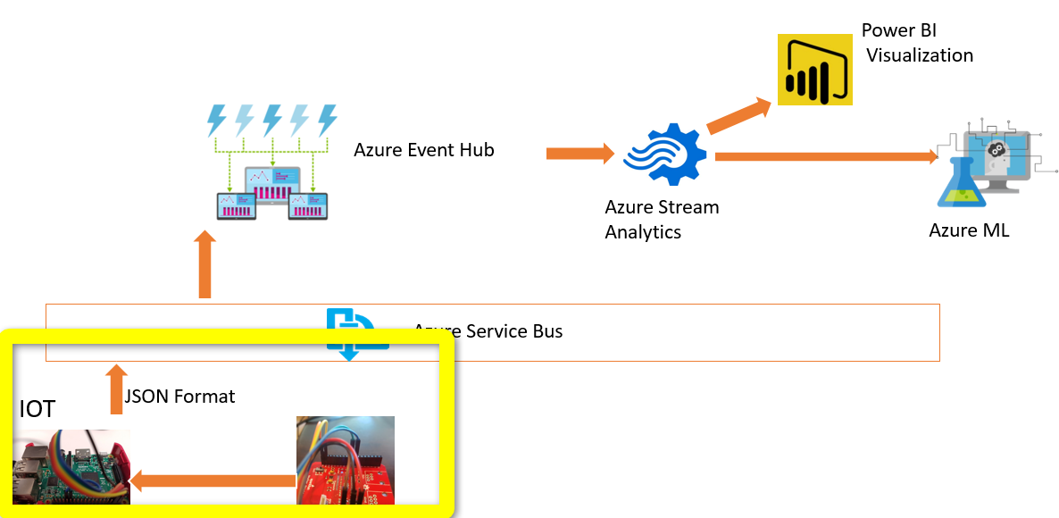
for this exmaple, lets’ have a look on the weather data, I have a post on IOT, which I fetch data from a sensor and show the live data in Power BI

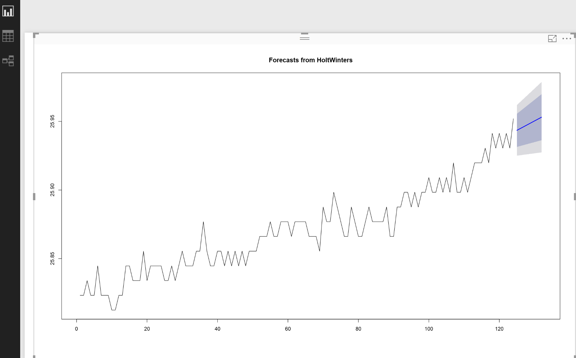
So every minutes I have about 30 data point about the temreture of the room. I want to forecast the weather tempreture for last 16 seconds later.
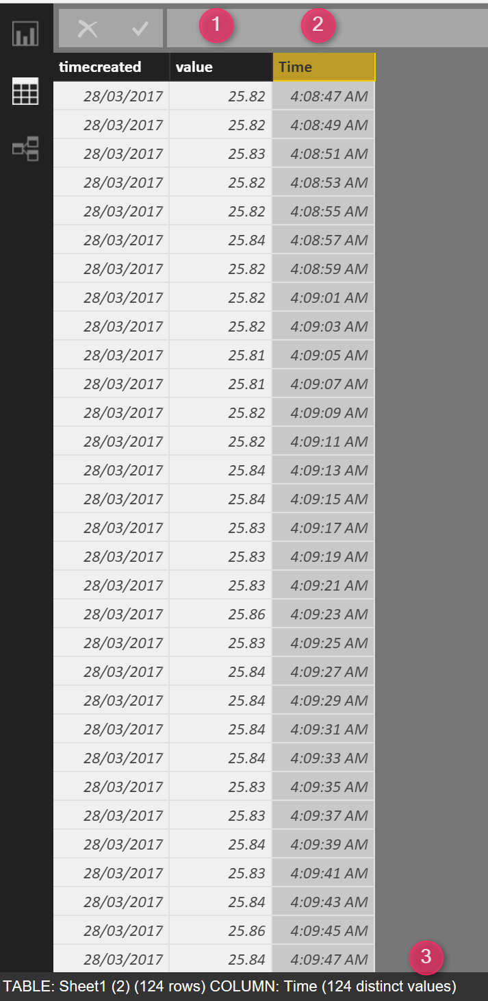
I have a dataset as below , the value for the tempreture, the time that is start from 4:08:47 am then it continues for 124 different second (number 3) as below :
So in Power BI, I am going to first shows the data in a time series object usingthe below codes
Tempts<-ts(dataset[2],start=c(1))
plot.ts(Tempts)
So I have a dataset, I consider the start as 1 that is the first minute, then I just convert the dataset into a timeseries object
then I used the plot function to draw it as below:
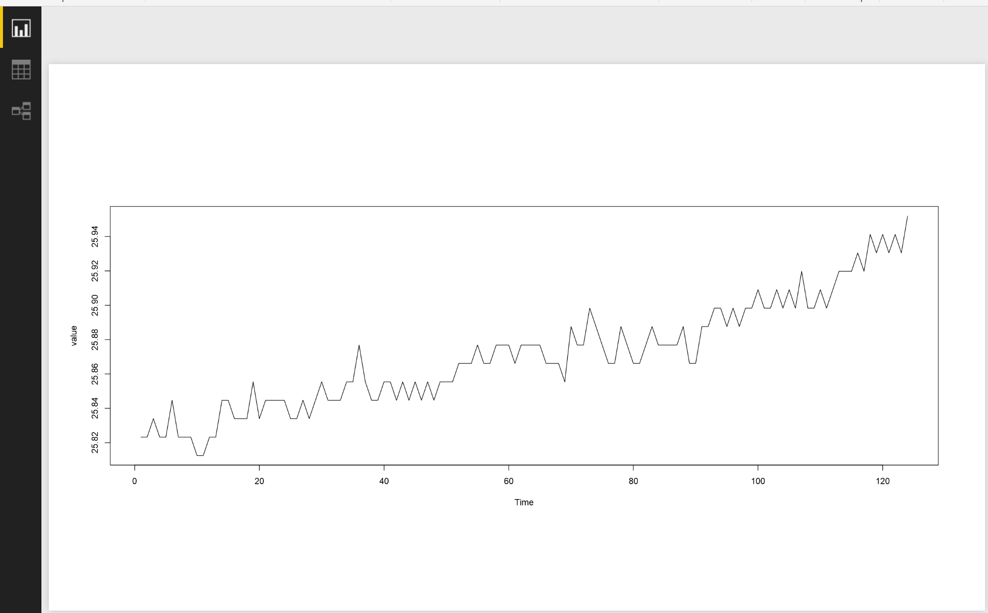
So as you can see in the above picture there is no seasonality pattern there, but there is a “an increase trend” there.
For this post, we have both Alfa and Beta value (Beta was for trend Data). but we donot have Gamma that is for checking the dependancy of seasonality to previouse time. as we donot have any seasonality in the data as you can see in above picture, so gamma value should be false. I am going to use the same function I had in “Simple Exponential Smoothing” name as “HoltWinters” such as below:
TempTrend<-HoltWinters(Tempts, gamma=FALSE)
The rest is the same as last post, I need library “forecast” and I am going to use the forecast function to forecast the value
Tempts<-ts(dataset[2],start=c(1))
#plot.ts(Tempts)
TempTrend<-HoltWinters(Tempts, gamma=FALSE)
library(forecast)
TempTrendforecasts <- forecast.HoltWinters(TempTrend, h=8)
plot.forecast(TempTrendforecasts )
I am going to forecast the value fore the next 8 points (every 2 seconds), so for nect 16 seconds I am going to predict the value
So the above chart will be shown.
Imagin that you are not interested to see the result in R visual, and only interested to see the result in Power query, so I am going to show the result in the power query as below :
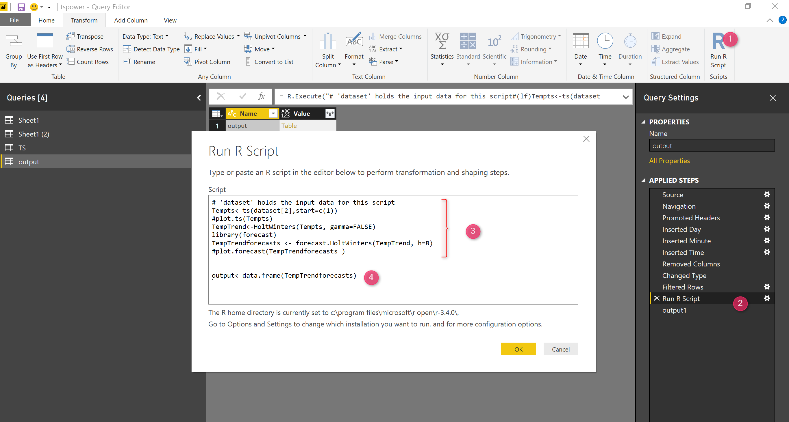
As you can see in the above code, In power query, I just clicked on the “R transfomr” on my dataset, then I just copy and past the code I have in the r visual, just comment the plot functions.
Then in number 4, I added a simple R codes to be able to show the result as a separate query by converting the result into data.frame into a varibale name “output”:
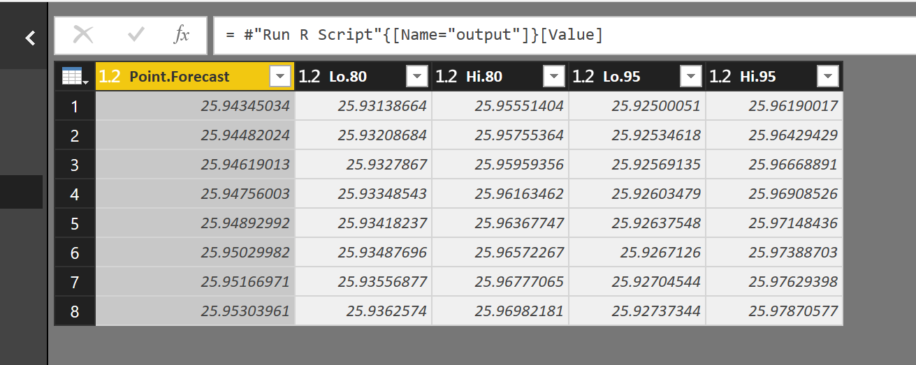
so the result for next 16 second can be shown as a separate query.
The first column is the forecast value, the second and third column it is show the upper and lower level for 80% and the forth and fifth shows the value for 95%.
In the next Posts, I will talk about, if we have seasonality and the correlation for errors.
[1]Book:http://a-little-book-of-r-for-time-series.readthedocs.io/en/latest/src/timeseries.html