
One of the most common types of banding or binning is banding based on a range. Let’s say, for example, you want to have a group of customers based on their age group. The age group banding can be created in Power Query at the data transformation stage. It can be created using the Grouping and Binning option in Power BI, or it can be even created using DAX measures. If you use a DAX measure for the banding, then TREATAS can be a useful function for implementing it. In this post, I’ll explain how it works.
If you are New to TREATAS
If you haven’t use TREATAS before and are new in using this function, I do recommend reading/watching the first two articles that I explained the way that TREATAS works;
Building a Virtual Relationship in Power BI – Basics of TREATAS DAX Function
Creating Relationship Based on Multiple Fields in Power BI Using TREATAS DAX Function
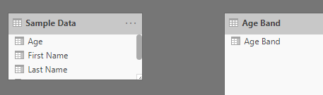
Sample Model
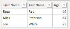
I am using a very simple data model in this example, the table below is what I use as the Sample Data;
Sample Data =
DATATABLE(
     'First Name',STRING,
     'Last Name',STRING,
     'Age',INTEGER,
     {
         {'Reza','Rad',40},
         {'Mick','Peterson',34},
         {'Joe','White',23}
     }
)
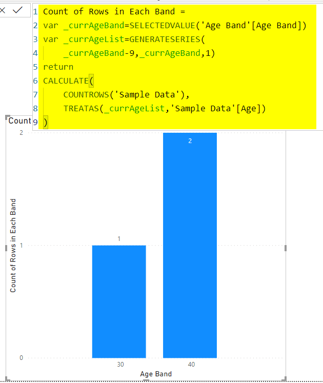
The goal is to have an age group banding for customers and get a count of customers in each group. something similar to this:

Other Methods for Banding
You can use Power Query with a conditional column to create banding, or you can use grouping and binning option in Power BI to achieve the same. Here, in this article, however, I am going to explain how that is possible through a measure using the TREATAS function.
Age Band Table
As we need the banding to be the axis of the chart, we need that as a field, You can create an age band table using What-If parameters, using the GenerateSeries function, or simply using an expression like this:
Age Band =
DATATABLE(
    'Age Band',INTEGER,
    {
        {10},{20},{30},{40}
    }
)
here is how the Age Band table looks like:
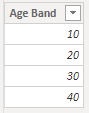
when you see 10 as the band up there, it means from 1 to 10, when you see 20, it means from 11 to 20 and so on.
This table shouldn’t have a relationship with the Sample Data table, because if you create the relationship, then it would only filter data for the top value of each band. so the tables remain unrelated. like a normal way of using a What-if parameter table.
DAX Measure using TREATAS
Now, using a measure like below, we can get the count of people in each band;
Count of Rows in Each Band =
var _currAgeBand=SELECTEDVALUE('Age Band'[Age Band])
var _currAgeList=GENERATESERIES(
    _currAgeBand-9,_currAgeBand,1)
return
CALCULATE(
    COUNTROWS('Sample Data'),
    TREATAS(_currAgeList,'Sample Data'[Age])
)
The expression can be split into multiple sections. First is the variable that fetches the current age band (the age band in the visualization’s filter context);
var _currAgeBand=SELECTEDVALUE('Age Band'[Age Band])
Then the next variable is a list (table) of values from the selected age band minus nine, to the value itself, increasing one at a time. for example; if age band value is 40, this list would be from 31 to 40: 31, 32, 33, …., 40.
var _currAgeList=GENERATESERIES(
    _currAgeBand-9,_currAgeBand,1)
Now that we have a list of possible age values for this band, we can use that to filter the Sample Data table using TREATAS;
CALCULATE(
    COUNTROWS('Sample Data'),
    TREATAS(_currAgeList,'Sample Data'[Age])
)
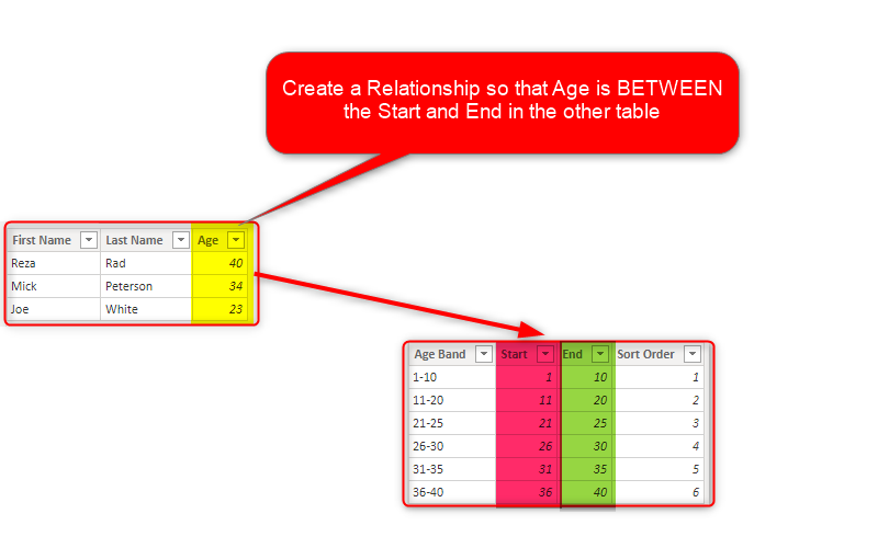
Altogether, this works like a scenario that you have created a relationship between the Age Band table and the Sample Data but on a BETWEEN condition, not an exact equal condition.
This example shows a really interesting use case for TREATAS, which is creating a relationship based on not-equal criteria. Relationships in Power BI are on the basis of equality of values, you cannot create a relationship that says this value should be less than or equal, or between or anything like that of the other value in the other table. However, using TREATAS combined with other functions, you can do that. I’ll write about this design pattern separately later in detail.
Age Bands with Start and End
If we step beyond the basic example, we can even create a bit more advanced banding. One of the limitations of grouping and binning in Power BI is that bins should be all of the equal size. For example, all age bands should be of 10 years, or all 5 years, you cannot say some are smaller than the others. Using your own Age Band table, however, you can define exactly what you want. Here is another detailed Age Band table;
Age Band Detailed =
DATATABLE(
    'Age Band',STRING,
    'Sort Order',INTEGER,
    'Start',INTEGER,
    'End',INTEGER,
    {
        {'1-10',1,1,10},
        {'11-20',2,11,20},
        {'21-25',3,21,25},
        {'26-30',4,26,30},
        {'31-35',5,31,35},
        {'36-40',6,36,40}
    }
)
and the table looks like this:
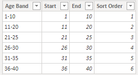
As you see, I have bands which are only covering five years (31-35), and bands that are covering ten years (11-20).
DAX Measure For Custom Bands
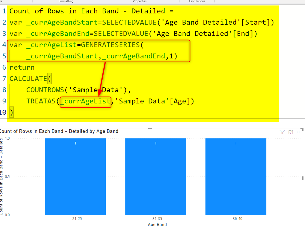
The DAX calculation is very similar to the previous one, the only difference is that we do not need to go nine years back, we have the start and end, and can generate the period using those;
Count of Rows in Each Band - Detailed =
var _currAgeBandStart=SELECTEDVALUE('Age Band Detailed'[Start])
var _currAgeBandEnd=SELECTEDVALUE('Age Band Detailed'[End])
var _currAgeList=GENERATESERIES(
    _currAgeBandStart,_currAgeBandEnd,1)
return
CALCULATE(
    COUNTROWS('Sample Data'),
    TREATAS(_currAgeList,'Sample Data'[Age])
)
The result is as below;
Creating the Relationship Based on Between
Age banding and grouping here was just an example to show the main pattern. The pattern is whenever you want to create the relationship between two tables based on a condition that is not Equal, but it is between, how you can do it.
The trick to do this pattern of creating a relationship based on between criteria is to use a function such as GenerateSeries to build a list of possible values between the two ends of each band, and then use it in TREATAS (or any other filter functions) to filter the value in the other table. That is what you see highlighted in the expression above.
Download Sample Power BI File
Download the sample Power BI report here:
Video


Reza is author of more than 14 books on Microsoft Business Intelligence, most of these books are published under Power BI category. Among these are books such as Power BI DAX Simplified, Pro Power BI Architecture, Power BI from Rookie to Rock Star, Power Query books series, Row-Level Security in Power BI and etc.
He is an International Speaker in Microsoft Ignite, Microsoft Business Applications Summit, Data Insight Summit, PASS Summit, SQL Saturday and SQL user groups. And He is a Microsoft Certified Trainer.
Reza’s passion is to help you find the best data solution, he is Data enthusiast.
His articles on different aspects of technologies, especially on MS BI, can be found on his blog: https://radacad.com/blog.