
 In the last post , I have explained the main concepts behind the timeseries. In this post, I am going to show how we can forecast for some periods. In the last post, I have mentioned that there is a possibility to have “seasonality” “Trend” and errors (residual) in one dataset: Seasonality+Trend+Residual we call it as an additive model [2] the first approach that I am going to talk is about ” Exponential Smoothing” Exponential Smoothing (ES) can be used for below scenarios
1-Simple (ES):
having an additive model with a constant level and no seasonality that is used for short term forecast. before showing how we can use this method for forecasting let me discuss some approaches. The first approach is very simple one name Naive Approach
“Naive approach” [4]
Imagin we have data series as :[ 10,13,23,23,24,23], So what s the next Value? the easy way is to say after 23 we will have just 24! so it is like just look at the one step before! not more : Yt=Yt-1 
Simple Average
Another approach is to consider more relevant time in the past and see that in average how much value we have so predict in future we will have the same! such as :[ 10,13,23,23,24,23], in average I can said the next value is 19! so we have below formula: 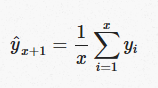 The next one is Moving Average
Moving Average
However, the last two approach is not complete is not wise at all just look at the last month rain and predict this month, also it is not good idea to take the average of rainfall for all years and predict the next month, maybe combination of these approaches be good, that means recent month rain fall or recent years rain fall value matter, so instead of considering all 10 years rainfall, it is better to just consider last 2 years average so in our example would be : :[ 10,13,23,23,24,23] 23,24,23 average will be 23
Weighted Moving Average
However, we can have some more accurate approach by considering the impact of recent month higher than later one, for instance the possibility that the current week weather islike last week is higher than to be same as last month. so in our example :[ 10,13,23,23,24,23] the weight for last value (23) can be 80%, for second last (24) would be 70% for third last (23) would be 60% and so on so we have below (23*0.8)+(24*0.7)+(23*0.6)+(23*0.5)+(13*0.4)+(10*0.3)/6=12 However, Single Exponential Smoothing follow the last approach with some changes,
Single Exponential Smoothing
so here we have Alfa value as weighted for the time, so if we consider the weight for the last month (July) is 0.9 for June would be 0.9^2, for May would be 0.9^3. so if we have just two months then Y july =alfa *Y july +(1-alfa)*Y august or in simple Y july =0.9 Y july +0.1 Y august 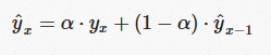
Example
We are going to forecast the amounth of annual rainfalls from 1813 to 1912 (100 years in London)[2] 
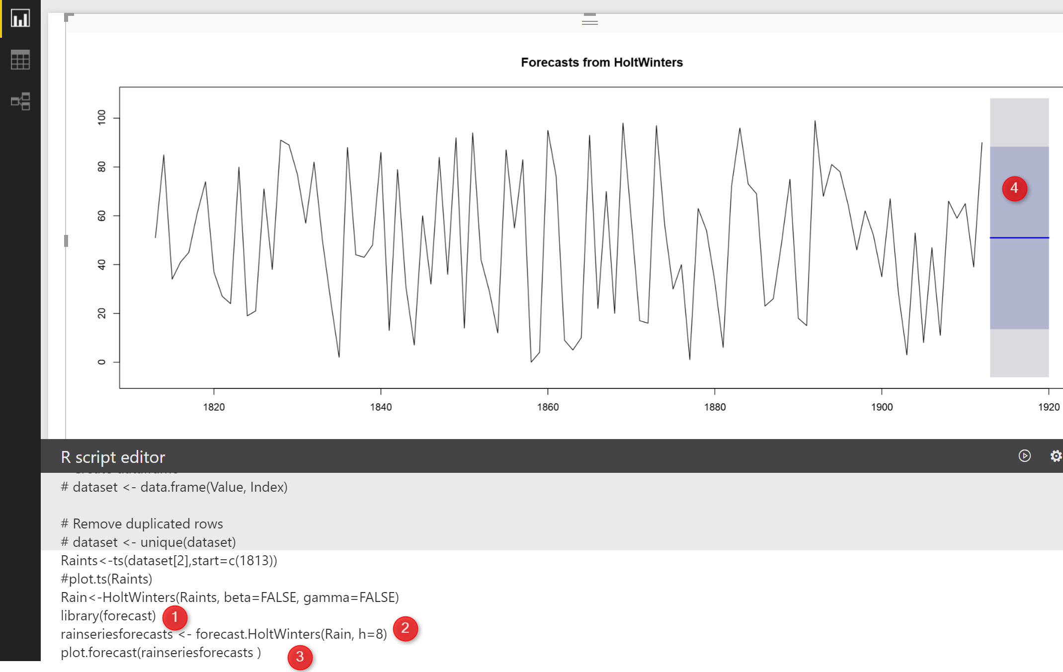
 In power BI, I am going to draw this data. First, I am going to convert it to Timeseries object, we imported the data into Power BI and put a R code inside the report area, then in R editor I wrote the below codes:
Raints<-ts(dataset[2],start=c(1813))
plot.ts(Raints)
So I got the below Plot 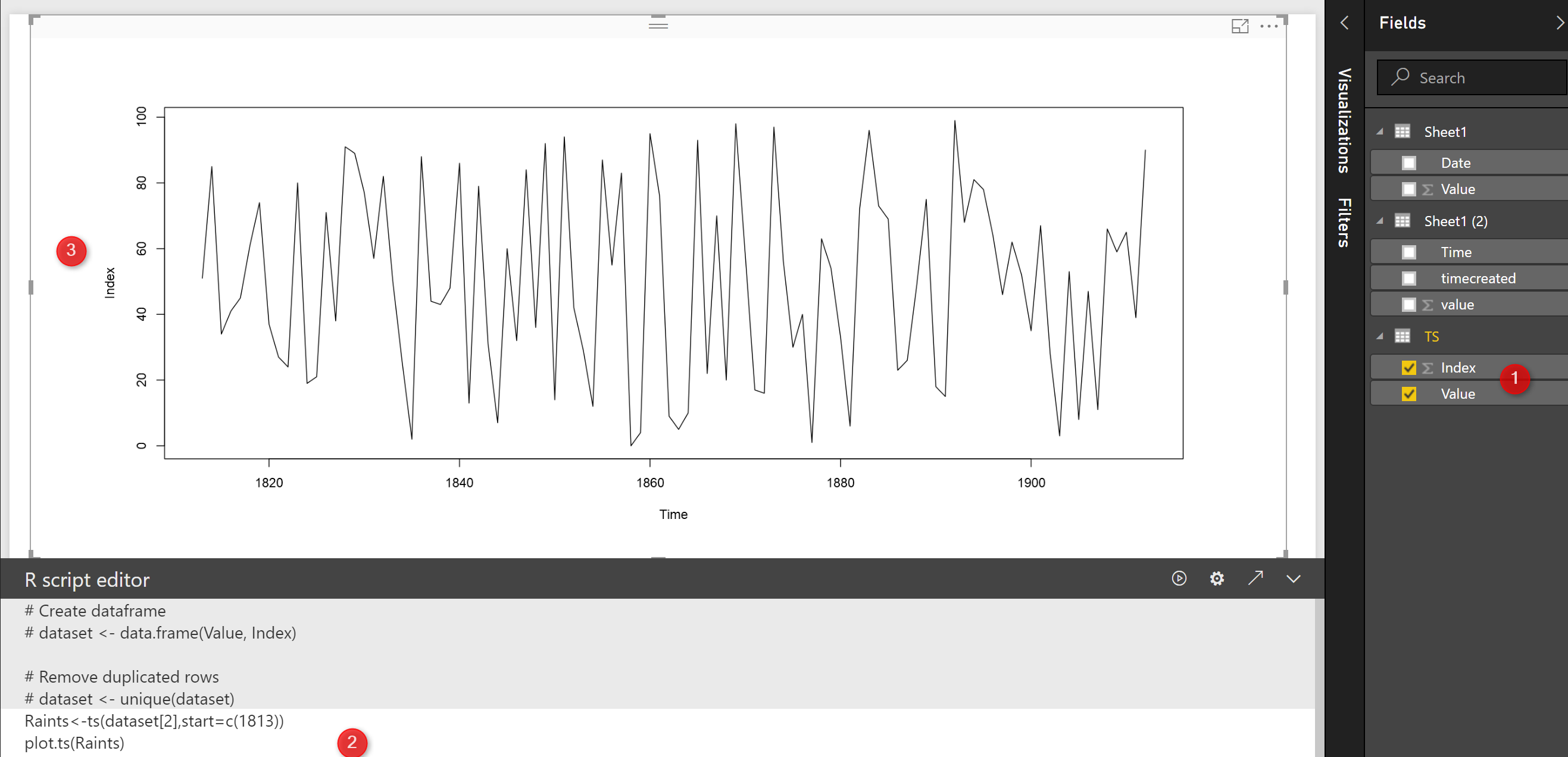 As you can see in the above picture, there is no seasonality in the rainfall data, also there is no trend (decrease or increase), it is all fluctuate around 60, so this is a good example that we can use simple exponential smoothing for forecasting. I am going to call function HoltWinters as below:
Rain<-HoltWinters(Raints, beta=FALSE, gamma=FALSE)
This method we look at the previous data point we have, this function gets below input[3]: First Input: The Timeseries Object, that we already created in the last step and store it in “Raints” Object. Second input: Beta, the Beta value is related to the data that has Trend (we do not have any trend in this example!) Beta has a degree that tells the system, how much focus on the recent changes in trend. in this example, we put Beta as false becuase we donot have any trend. Gamma, related to the seasonal component, higher gamma means the more recent seasonal component is weighted. in this example, we don’t have any seasonality, so we put the(Gamma) third parameter as False. So we have below code. However, I want to see the values for Rain variable, I just click on the arrow at the right side of R editor (number 2) to open the code inside the R studio.  I have below in Rstudio
 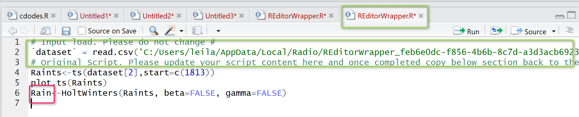 Now if I just Run the “Rain” (Below pic number 1) variable
 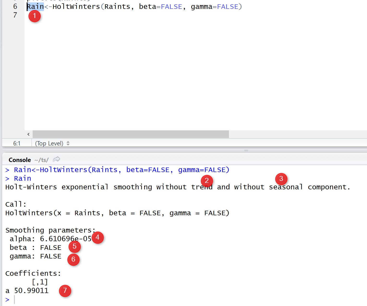 as you see the result of the run, there are comments that said “there is no trend or seasonality” also, we have value as6 for Alfa, (I have explained the Alfa value) higher Alfa means the time series is more related to the recent numbers than the later one. Now, I am able to forecast the rain by using a function name “Forecast”. the function gets the output of the Exponential Smoothing (HoltWinters) and the period that we want to forecast.
rainseriesforecasts <- forecast.HoltWinters(Rain, h=8)
to call this function we need a library as “library(forecast)” and also to plot the result we need another function as plot.forecast() so the result would be as below as you see in above picture the constant value has been predicted for 8 years as 50 I will discuss how to find the accuracy and errors in next post.
[1] Book:http://a-little-book-of-r-for-time-series.readthedocs.io/en/latest/src/timeseries.html
[2]http://www-ist.massey.ac.nz/dstirlin/CAST/CAST/Hmultiplicative/multiplicative1.html
[3]http://www.scmfocus.com/demandplanning/2011/03/alpha-beta-and-gamma-in-forecasting/
[4] https://grisha.org/blog/2016/01/29/triple-exponential-smoothing-forecasting/