Neural Network R codes in Power BI Part2

In the last post, I have explained the main concepts behind the neural network,

In this post I will show how to apply neural network in a scenario in R and how to see the results and hidden layers in a plot.

For this post I got some great example from [1].

Scenario:

Concert has been use in many different structure such as bridge, apartment, roadways and so on.

For the safety the strength of the concrete is matter. the concrete strength depends on the material that have been used to create it such as :Cement, Slag, Ash, water, and so forth.

imaging that we have a dataset as below, which shows the ingredient of concrete.

we are going to predict the concrete strength using neural network. neural network can be used for predict a value or class, or it can be used for predicting multiple items. In this example, we are going to predict a value, that is concrete strength.

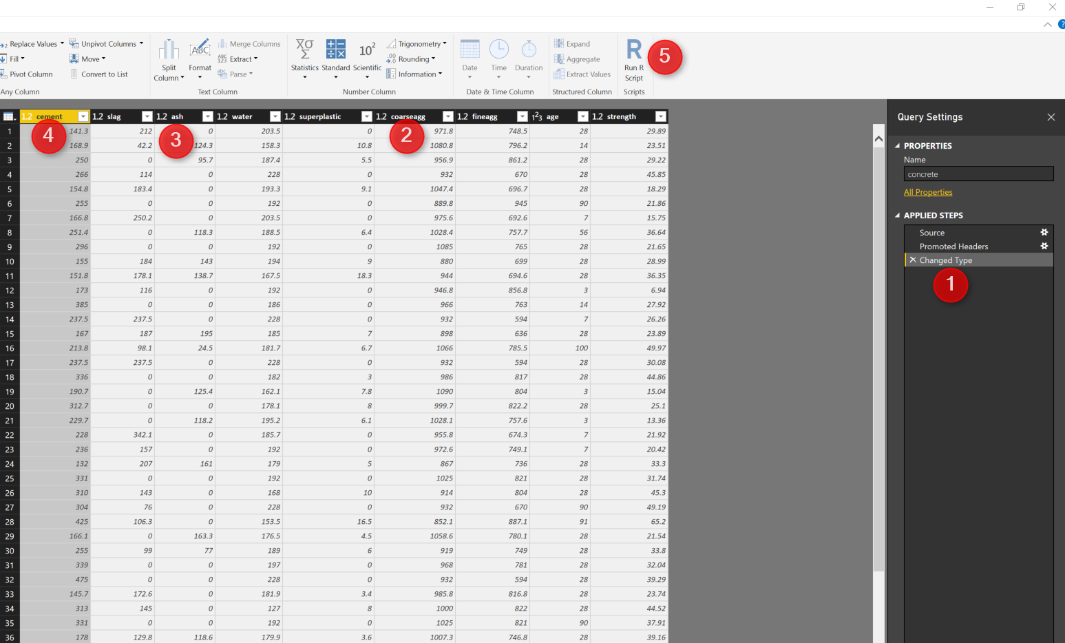
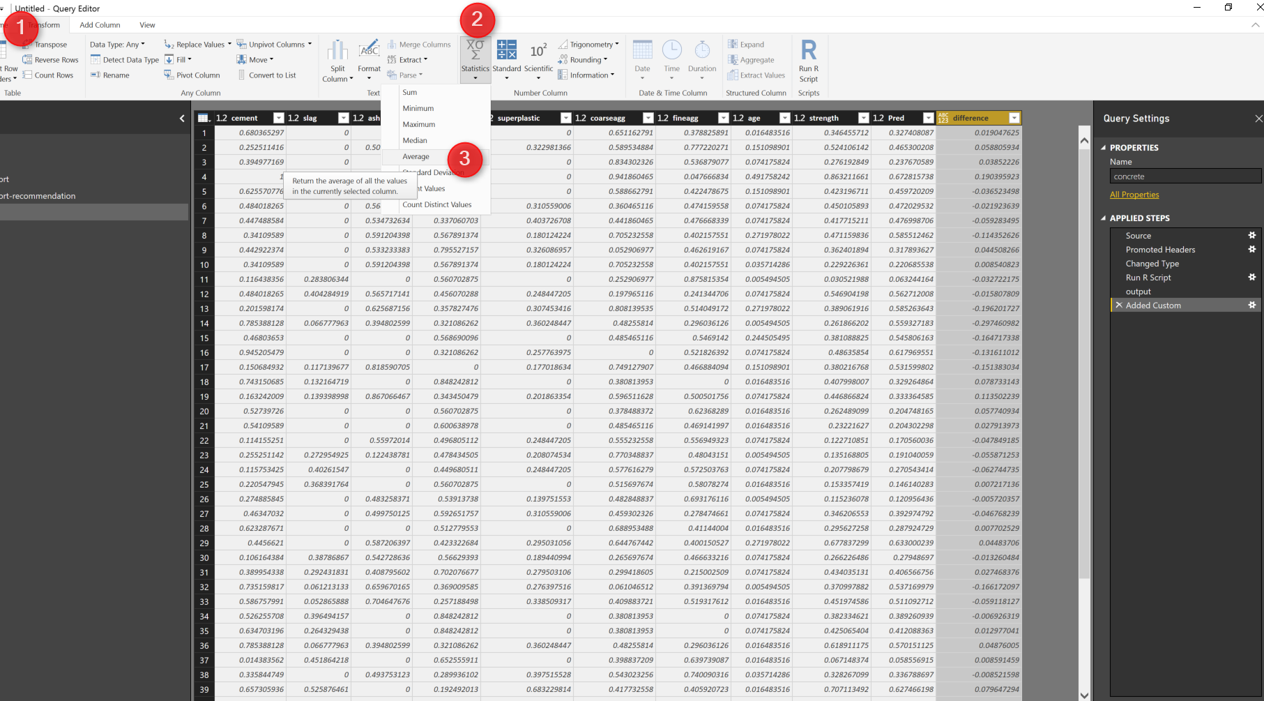
I have loaded the data in power bi first, and in “Query Editor” I am going to write some R codes. First we need to do some data transformations. As you can see in the below picture number 2,3 and 4,data is not in a same scale, we need to do some data normalization before applying any machine learning. I am going to write a code for that (Already explained the normalization in post KNN). So to write some R codes, I just click on the R transformation component (number 5).

I have used the below codes to normalized the dataset.

normalize <- function(x) {
    return((x - min(x)) / (max(x) - min(x)))
}

concrete_norm <- as.data.frame(lapply(dataset, normalize))

The same as any predictive model first we should provide some set of data for training and the other for testing as below.

concrete_train <- concrete_norm[1:773,]
concrete_test <- concrete_norm[774:1030,]

Next, I am going to call a package for Neural network that has been used a lot, name as “neuralnet”. There are other packages for this purpose. I first install it using intall.packages command in my Rstudio.

library("neuralnet")
	concrete_model <- neuralnet(strength ~ cement + slag
	+ ash + water + superplastic + coarseagg + fineagg + age,
	data = concrete_train)

This package has a function name (neuralnet) that create a model.

next, I am going to run the model against the training dataset for all 8 attributes as below

model_results <- compute(concrete_model, concrete_test[1:8]) 
predicted_strength <- model_results$net.result

finally I create an output data frame dataset to show the result in Power BI

output<-dataset[774:1030,]
output$Pred<-predicted_strength

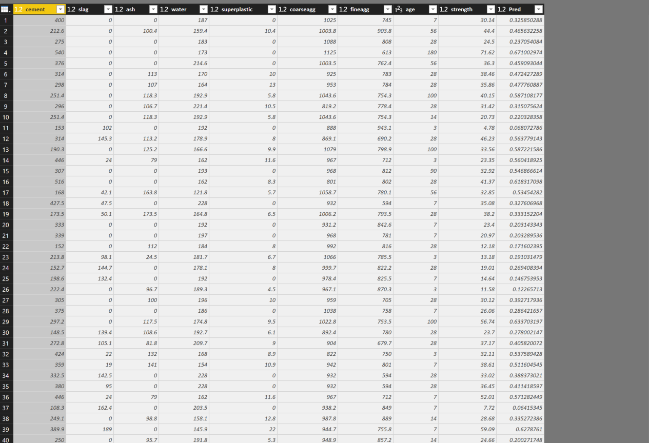
The output has been shown in the below picture. column 9 (strength) shows the real concrete strength, while the column 10 (pred) shows the prediction from neural net.

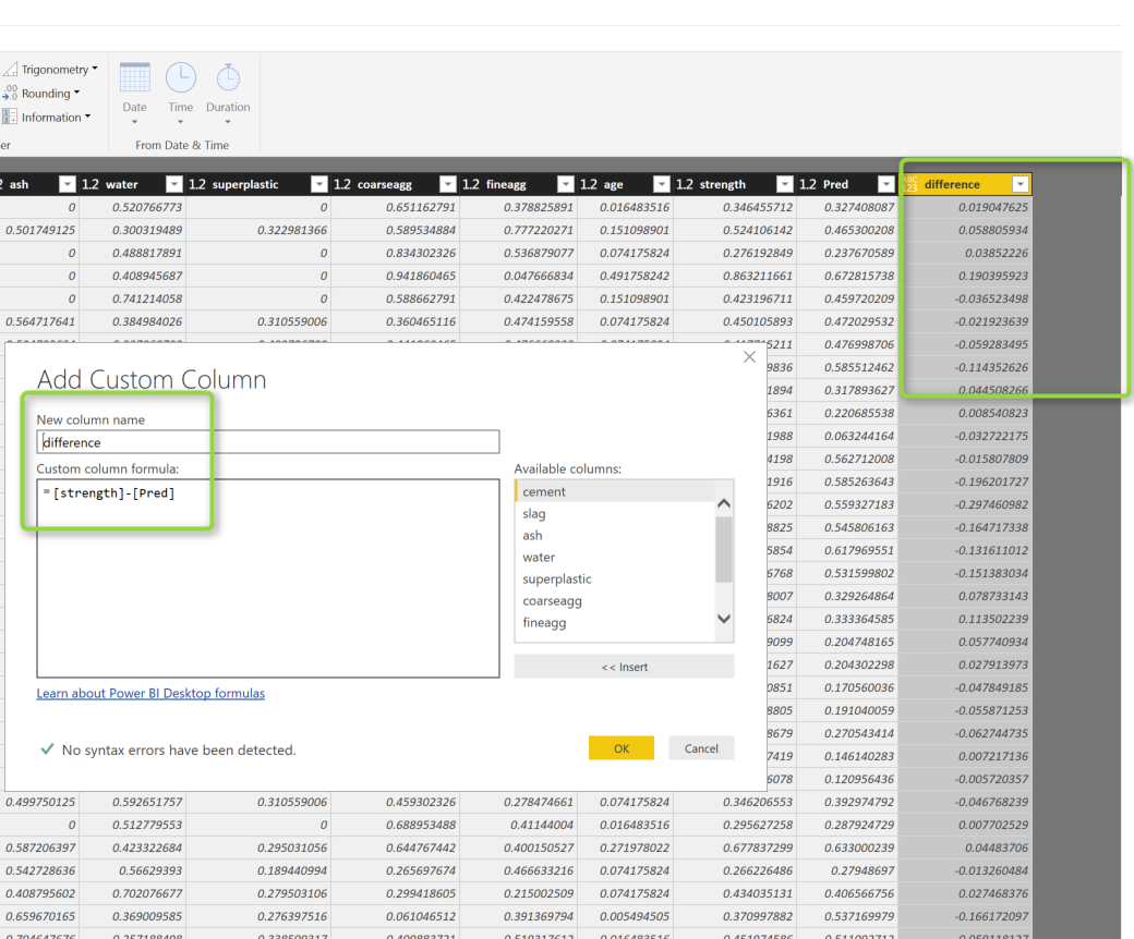
I created a custom column to see the differences between predicted and the orinal value

as you see in below picture:

the differences are not that much, and if you just go to transform (number 1 in the below picture) and then choose the Average (number 2 and 3)

you will see the difference is not that much in average=-0.0044

which shows the prediction is good

However, you may interested to see the plot in visualization and see the hidden nodes and other information like weights.

so I am going to report area and just copy and paste the code I run for the neural network

normalize <- function(x) {
    return((x - min(x)) / (max(x) - min(x)))
}

concrete_norm <- as.data.frame(lapply(dataset, normalize))
summary(concrete_norm$strength)
concrete_train <- concrete_norm[1:773,]
concrete_test <- concrete_norm[774:1030,]
library("neuralnet")
	concrete_model <- neuralnet(strength ~ cement + slag
	+ ash + water + superplastic + coarseagg + fineagg + age,
	data = concrete_train)

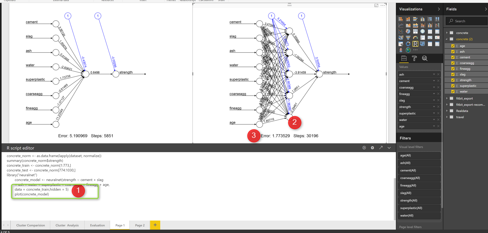
just I add plot to show the model

plot(concrete_model)

the output will be like :

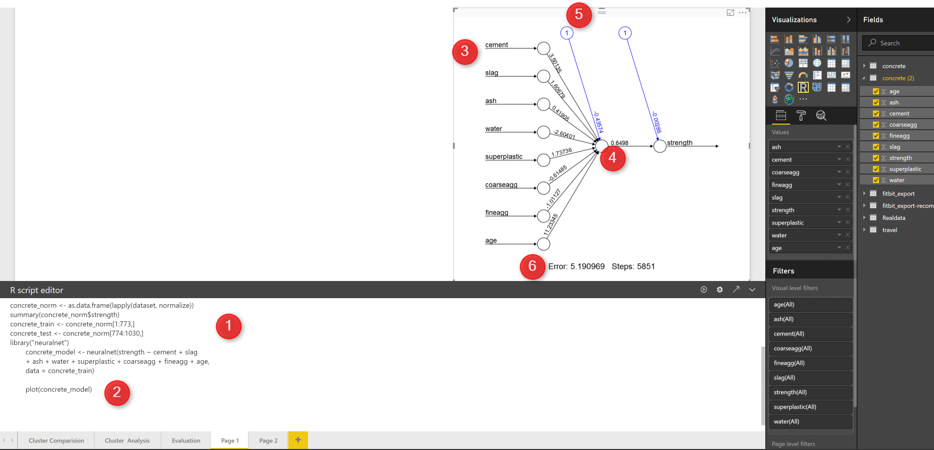
as you can see in the above picture, in number 1, I just copy and past the code (I change the dataset name). then I simply use the plot (number 2) to show the neural network.

you see the net work structure in visualization section. The number 3 show the input that we consider to predict the strength of the concrete. number 5 is a intercept or biased number. number 4 is the strength weight. and in number 6 at the bottom of the page you will the error and how many steps has gone to reach. this is a very simple network, just one hidden node, lets add some hidden node to this model just by changing the code  as below :

concrete_model <- neuralnet(strength ~ cement + slag
	+ ash + water + superplastic + coarseagg + fineagg + age,
	data = concrete_train,hidden = 5)

The only changes is to add parameter “Hidden” to the neural net function (number 1).  then just run the code and you will see another network that has 5 different hidden node. and if you look at the error, you will see it decrease so much! so always having some more hidden layer can be helpful but not that much, I could not find a rule to identify number of hidden node, but if you have any hidden node then we have the problem of over fitting see related post about over fitting

[1]Machine Learning with R,Brett Lantz, Packt Publishing,2015

Leila Etaati

Trainer, Consultant, Mentor

Leila is the first Microsoft AI MVP in New Zealand and Australia, She has Ph.D. in Information System from the University Of Auckland. She is the Co-director and data scientist in RADACAD Company with more than 100 clients in around the world. She is the co-organizer of Microsoft Business Intelligence and Power BI Use group (meetup) in Auckland with more than 1200 members, She is the co-organizer of three main conferences in Auckland: SQL Saturday Auckland (2015 till now) with more than 400 registrations, Difinity (2017 till now) with more than 200 registrations and Global AI Bootcamp 2018. She is a Data Scientist, BI Consultant, Trainer, and Speaker. She is a well-known International Speakers to many conferences such as Microsoft ignite, SQL pass, Data Platform Summit, SQL Saturday, Power BI world Tour and so forth in Europe, USA, Asia, Australia, and New Zealand. She has over ten years’ experience working with databases and software systems. She was involved in many large-scale projects for big-sized companies. She also AI and Data Platform Microsoft MVP. Leila is an active Technical Microsoft AI blogger for RADACAD.